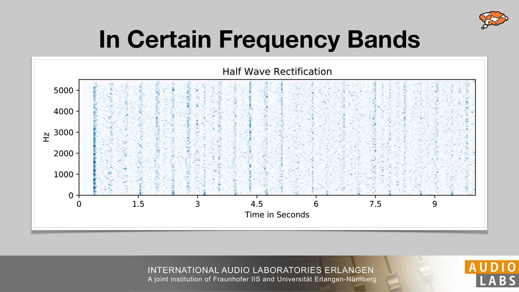
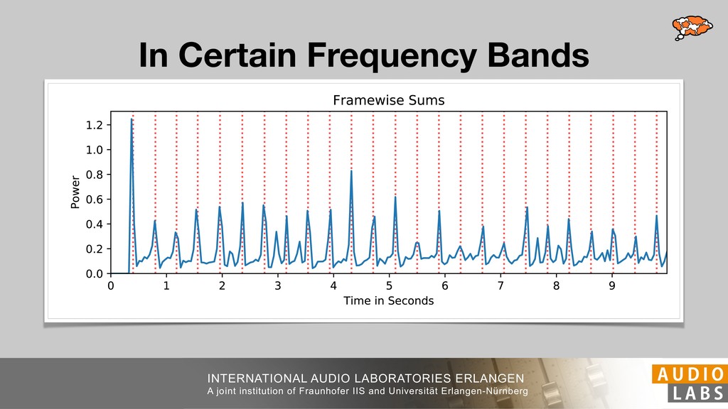
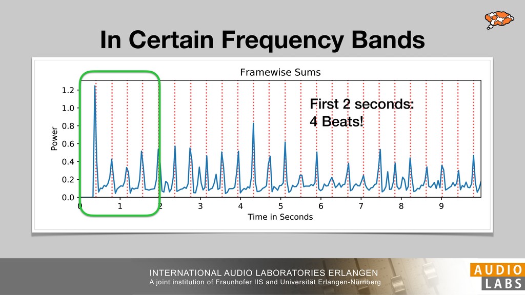
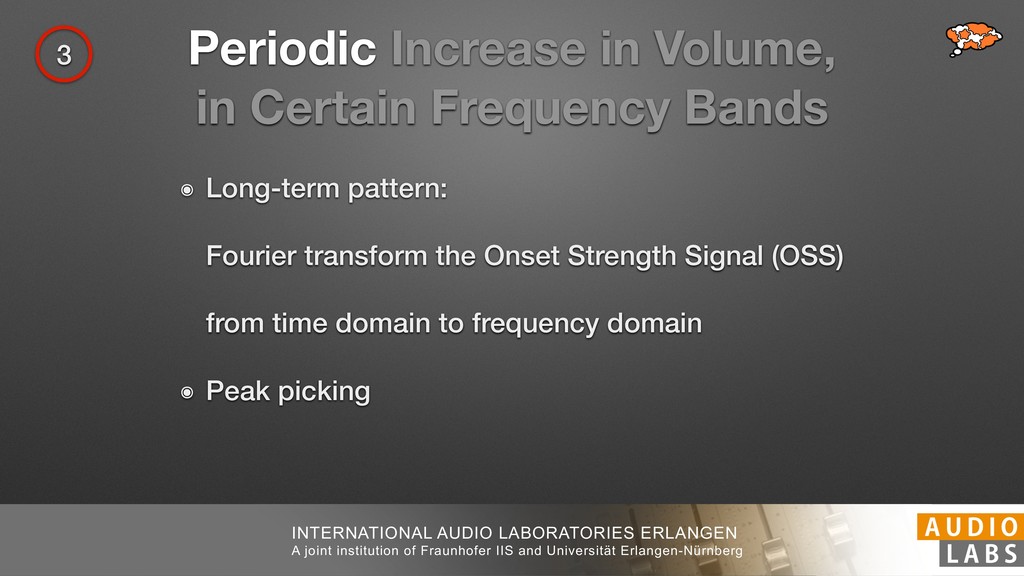
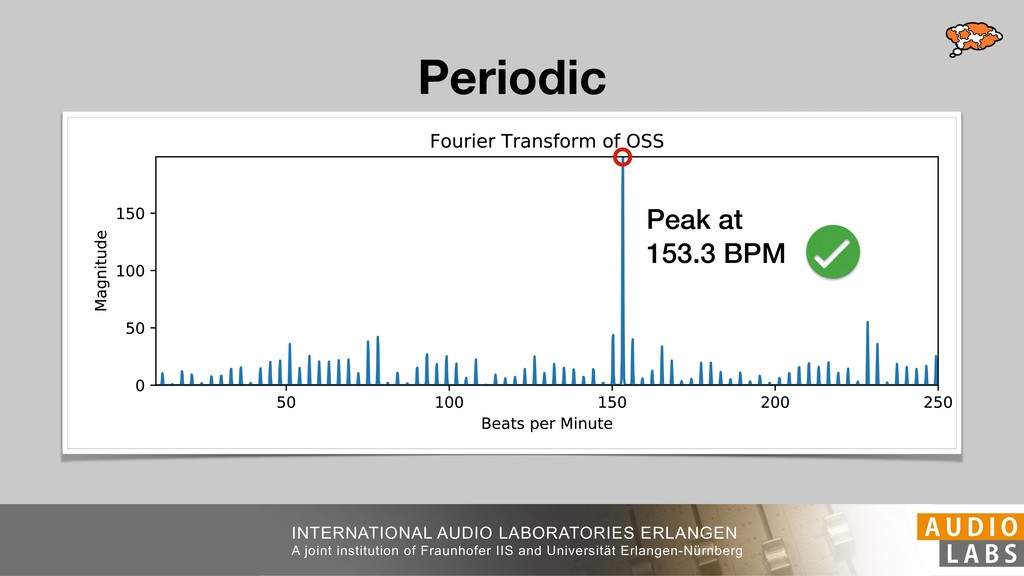
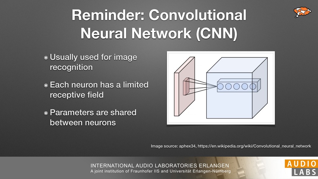
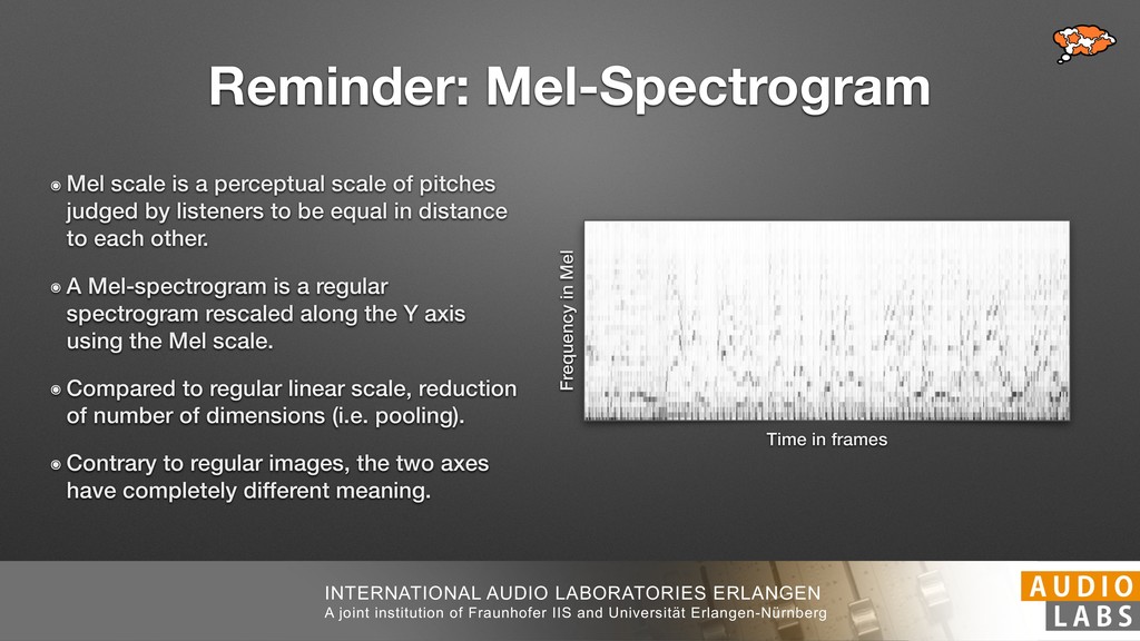
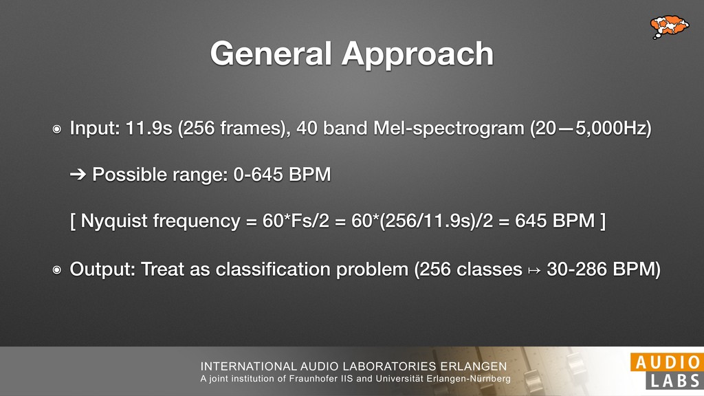
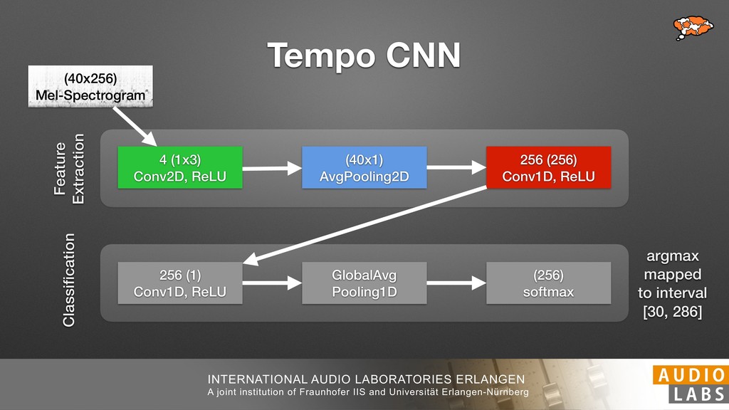
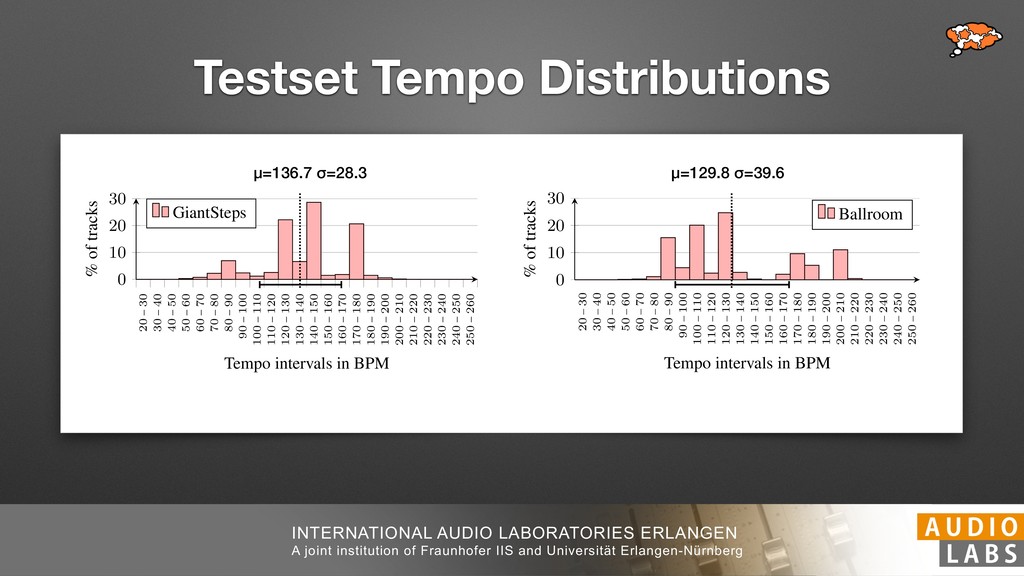
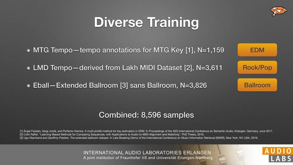
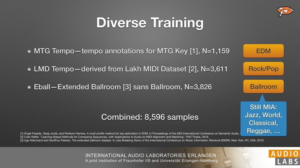
and Universität Erlangen-Nürnberg Tempo Distributions tures, and then compare our results with those from other methods. Finally, in Section 5, we present our conclusions. 2. TEMPO ESTIMATION To lay the groundwork for our error correction method, we first describe a simple tempo estimation algorithm, then in- troduce several test datasets and discuss common pitfalls. In Section 2.5, we introduce performance metrics and de- scribe observed errors. 2.1 Algorithm To estimate the dominant pulse we follow the approach taken in [24], which is similar to [23, 28]: We first con- vert the signal to mono and downsample to 11025 Hz. Then we compute the power spectrum Y of 93 ms win- dows with half overlap, by applying a Hamming win- dow and performing an STFT. The power for each bin k 2 [0 : K] := {0, 1, 2, . . . , K} at time m 2 [0 : M] := {0, 1, 2, . . . , M} is given by Y (m, k), its positive logarith- mic power Yln (m, k) := ln (1000 · Y (m, k) + 1), and its frequency by F(k) given in Hz. We define the onset signal strength OSS(m) as the sum of the bandwise differences between the logarithmic powers Yln (m, k) and Yln (m 1, k) for those k where the frequency F(k) 2 [30, 720] 0 10 20 % of tr 0 10 20 30 % of tracks ISMIR2004 Songs µ = 89.80, = 27.83 N = 464 0 10 20 30 % of tracks GTZAN µ = 94.55, = 24.39 N = 999 0 10 20 30 % of tracks ACM MIRUM µ = 102.72, = 32.58 N = 1410 0 10 20 30 % of tracks Hainsworth µ = 113.30, = 28.78 N = 222 20 30 acks Ballroom µ = 129.77, = 39.61 mic power Yln (m, k) := ln (1000 · Y (m, k) + 1), and its frequency by F(k) given in Hz. We define the onset signal strength OSS(m) as the sum of the bandwise differences between the logarithmic powers Yln (m, k) and Yln (m 1, k) for those k where the frequency F(k) 2 [30, 720] and Y (m, k) is greater than ↵Y (m 1, k) (see [16]): I(m, k) = 8 < : 1 if Y (m, k) > ↵Y (m 1, k) and F(k) 2 [30, 720], 0 otherwise (1) OSS(m) = X k (Yln (m, k) Yln (m 1, k)) · I(m, k) Both the factor ↵ = 1.76 and the frequency range were found experimentally [24]. The OSS(m) is transformed using a DFT with length 8192. At the given sample rate, this ensures a resolution of 0.156 BPM. The peaks of the resulting beat spectrum B represent the strength of BPM values in the signal [7], but do not take harmonics into account [10, 21]. There- fore we derive an enhanced beat spectrum BE that boosts frequencies supported by harmonics: BE (k) = 2 X |B(bk/2i + 0.5c)| (2) 0 10 20 % of tr N = 222 0 10 20 30 % of tracks Ballroom µ = 129.77, = 39.61 N = 698 20 – 30 30 – 40 40 – 50 50 – 60 60 – 70 70 – 80 80 – 90 90 – 100 100 – 110 110 – 120 120 – 130 130 – 140 140 – 150 150 – 160 160 – 170 170 – 180 180 – 190 190 – 200 200 – 210 210 – 220 220 – 230 230 – 240 240 – 250 250 – 260 0 10 20 30 Tempo intervals in BPM % of tracks GiantSteps µ = 136.66, = 28.33 N = 664 Figure 1. Tempo distributions for the test datasets. highest value of BE , divide its frequency by 4 to find the first harmonic, and finally convert its associated frequency to BPM: 60 40 – 50 50 – 60 60 – 70 70 – 80 80 – 90 90 – 100 100 – 110 110 – 120 120 – 130 130 – 140 140 – 150 150 – 160 160 – 170 170 – 180 180 – 190 190 – 200 200 – 210 210 – 220 0 10 20 30 Tempo intervals in BPM % of tracks µ = 121.32, = 30.52 N = 8, 596 Figure 1: Tempo distribution for the Train dataset con- sisting of LMD Tempo, MTG Tempo, and EBall. sisting of multiple components (“layers”) that has evolved naturally. But to the best of our knowledge, nobody has replaced the traditional multi-component architecture with a single deep neural network (DNN) yet. In this paper we describe a CNN-based approach that estimates the local end, we estimated the tempo of the matched audio pre- views using the algorithm from [31]. Then the associated MIDI files were parsed for tempo change messages. If the value of more than half the tempo messages for a given preview were within 2% of the estimated tempo, we as- sumed the estimated tempo of the audio excerpts to be cor- rect and added it to LMD Tempo. This resulted in 3,611 audio tracks. We were able to match more than 76% of the tracks to the Million Song Dataset (MSD) genre annota- tions from [29]. Of the matched tracks 29% were labeled rock, 27% pop, 5% r&b, 5% dance, 5% country, 4% latin, and 3% electronic. Less than 2% of the tracks were labeled jazz, soundtrack, world and others. Thus it is fair to characterize LMD Tempo as a good cross-section of popular music. 2.2 MTG Tempo The MTG Key dataset was created by Faraldo [8] as a Proceedings of the 19th ISMIR Conference, Paris, France, September 23-27, 2018 99 Diverse μ=121.3 σ=30.5 μ=94.6 σ=24.4