[m] -0.0015 -0.001 -0.0005 0 0.0005 0.001 0.0015 y [m] -0.0015 -0.001 -0.0005 0 0.0005 0.001 0.0015 Entries 10004 Mean x 0.08502 Mean y 2.227e-06 Mean z 1.231e-06 RMS x 0.0006551 RMS y 0.0006156 RMS z 0.0006149 Entries 10004 Mean x 0.08502 Mean y 2.227e-06 Mean z 1.231e-06 RMS x 0.0006551 RMS y 0.0006156 RMS z 0.0006149 z-x-y distr., step 5 FinPhase3.h5 z [m] 3.084 3.085 3.086 3.087 3.088 x [m] -0.0015 -0.001 -0.0005 0 0.0005 0.001 0.0015 y [m] -0.0015 -0.001 -0.0005 0 0.0005 0.001 0.0015 Entries Mean x Mean y Mean z RMS x RMS y RMS z Entries Mean x Mean y Mean z RMS x RMS y RMS z z-x-y distr., step FinPhase . 8 / 51
big project: > 100 people, expensive, 700 m long • 1 Ångström • to reach target it is of crucial importance to attain “good” beam properties (e.g. narrow beam/small phase space volume) . 1http://www.psi.ch/swissfel/ 10 / 51
big project: > 100 people, expensive, 700 m long • 1 Ångström • to reach target it is of crucial importance to attain “good” beam properties (e.g. narrow beam/small phase space volume) . . Calls for optimization of Injector • Several conflicting objectives • Key technology: multi-objective optimization 1http://www.psi.ch/swissfel/ 10 / 51
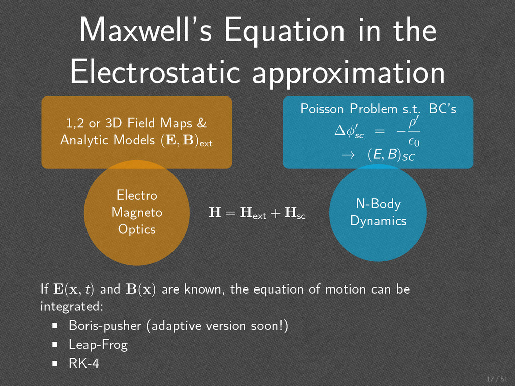
Optics . N-Body Dynamics . 1,2 or 3D Field Maps & Analytic Models (E, B)ext . Poisson Problem s.t. BC’s ∆ϕ′ sc = − ρ′ ϵ0 → (E, B)SC . H = Hext + Hsc . If E(x, t) and B(x) are known, the equation of motion can be integrated: • Boris-pusher (adaptive version soon!) • Leap-Frog • RK-4 17 / 51
latency with increasing # cores • Increasing congestion on links surrounding the master • Gets worse with increasing message sizes Flat network topologies not optimal Adapt number of masters depending on # cores Place master taking network topology into consideration Towards Message Passing for a Million Processes: Characterizing MPI on a Massive Scale Blue Gene/P, P. Balaji et. al. 22 / 51
for precise charged-particle optics in large accelerator structures and beam lines including 3D space charge. • built from the ground up as a parallel application • runs on your laptop as well as on the largest HPC clusters • uses the mad language with extensions • written in C++ using OO-techniques, hence OPAL is easy to extend • nightly regression tests track the code quality OPAL: https://amas.psi.ch/OPAL 29 / 51
# slices ≪ # macro particles • Slices distributed in contiguous blocks • Load imbalance of at most 1 slice • Low number of synchronization points 32 / 51
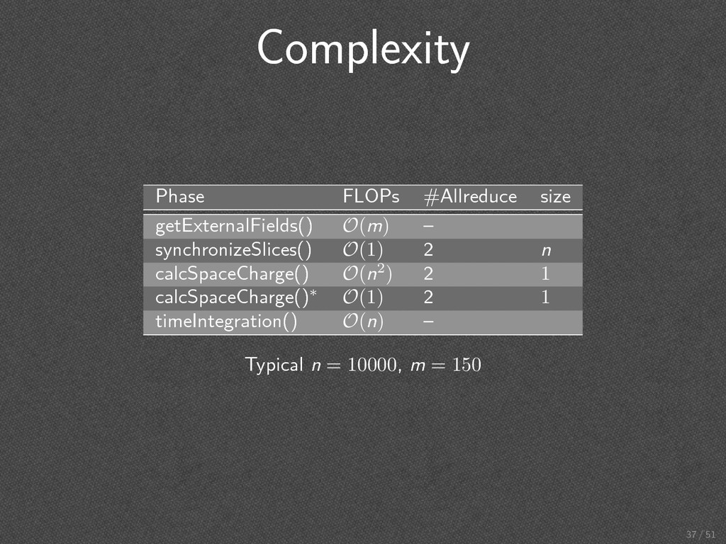
ti ∈ t1 , · · · , tn−1 , tn do 3: for all s ∈ slices do 4: getExternalFields(s) 5: end for 6: synchronizeSlices() 7: calcSpaceCharge() 8: for all s ∈ slices do 9: timeIntegration(s) 10: end for 11: end for 12: end procedure . 34 / 51
ti ∈ t1 , · · · , tn−1 , tn do 3: for all s ∈ slices do 4: getExternalFields(s) 5: end for 6: synchronizeSlices() 7: calcSpaceCharge() 8: for all s ∈ slices do 9: timeIntegration(s) 10: end for 11: end for 12: end procedure . 34 / 51
∈ my_slices do 3: for all j ∈ all_slices do 4: sm ← interaction(sj , si ) 5: end for 6: Fl,i ← longitudinalSpaceCharge(sm) 7: Ft,i ← transversalSpaceCharge() 8: end for 9: end procedure . 35 / 51
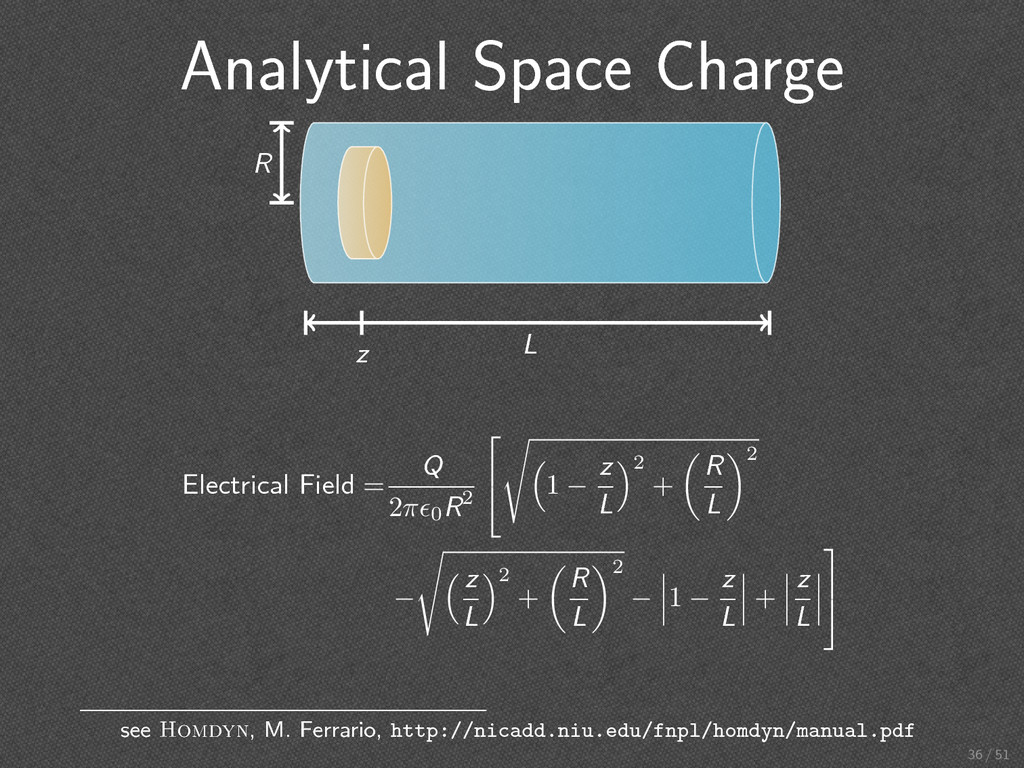
. z . . Electrical Field = Q 2πϵ0 R2 √ ( 1 − z L )2 + ( R L )2 − √ ( z L )2 + ( R L )2 − 1 − z L + z L see Homdyn, M. Ferrario, http://nicadd.niu.edu/fnpl/homdyn/manual.pdf 36 / 51
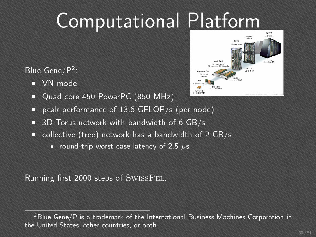
450 PowerPC (850 MHz) • peak performance of 13.6 GFLOP/s (per node) • 3D Torus network with bandwidth of 6 GB/s • collective (tree) network has a bandwidth of 2 GB/s • round-trip worst case latency of 2.5 µs Running first 2000 steps of SwissFel. . . 2Blue Gene/P is a trademark of the International Business Machines Corporation in the United States, other countries, or both. 39 / 51
Comm [s] 1 321.46 – 2 167.93 3.67 (2.19%) 4 92.9 6.86 (7.43%) 8 57.1 9.08 (15.91%) Run on FELSIM Cluster at PSI. • proper load balancing • profiling and benchmarking: serial parts (Amdahl’s law) • one fix synchronization point per timestep 40 / 51
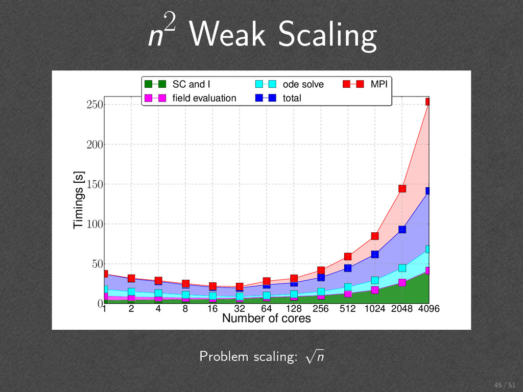
128 256 512 1024 2048 4096 Number of cores 0 50 100 150 200 250 Timings [s] SC and I field evaluation ode solve total MPI Problem scaling: n . . execisvely long MPI shutdown 44 / 51
low-dimensional model • almost 2 orders of magnitude reduction of runtime Crucial cornerstone of framework • becomes feasible with presented forward solver • vary “resolution” (3D, n2 sc., analytical sc.) • achieve an acceptable parallel efficiency for one forward solve • run as many parallel forward solves as possible Helps in design/opartion of particle accelerators 46 / 51
(βi Ri) + Ri ∑ j Kj i = 2c2kp Riβi × ( G(∆i, Ar) γ3 i − (1 − β2 i ) G(δi, Ar) γi ) + 4εth n c γi 1 R3 i d dt βi = e0 m0 cγ3 i ( Eext z (zi, t) + Esc z (zi, t) ) d dt zi = cβi 51 / 51
![Time Evolution z [m] 0.083 0.084 0.085 0.086 0.087 x](https://files.speakerdeck.com/presentations/4fea86ed1ce3a300220190ff/slide_7.jpg)
![Master/Worker Model Comp. Domain Optimizeri [coarse] multiple starting points, multiple](https://files.speakerdeck.com/presentations/4fea86ed1ce3a300220190ff/slide_22.jpg)
![First Population . . dE [MeV] . 0.20 . 0.22](https://files.speakerdeck.com/presentations/4fea86ed1ce3a300220190ff/slide_26.jpg)
![30th population . . dE [MeV] . 0.20 . 0.22](https://files.speakerdeck.com/presentations/4fea86ed1ce3a300220190ff/slide_27.jpg)
![649th Population . . dE [MeV] . 0.20 . 0.22](https://files.speakerdeck.com/presentations/4fea86ed1ce3a300220190ff/slide_28.jpg)
![“History” A stony road to achieve scalability.. Cores Wall [s]](https://files.speakerdeck.com/presentations/4fea86ed1ce3a300220190ff/slide_42.jpg)
![Optimization Problem min [energy spread, emittance] s.t. ∂t f(x, v,](https://files.speakerdeck.com/presentations/4fea86ed1ce3a300220190ff/slide_52.jpg)