Practical Image Classification & Object Detection

Abstract
--------
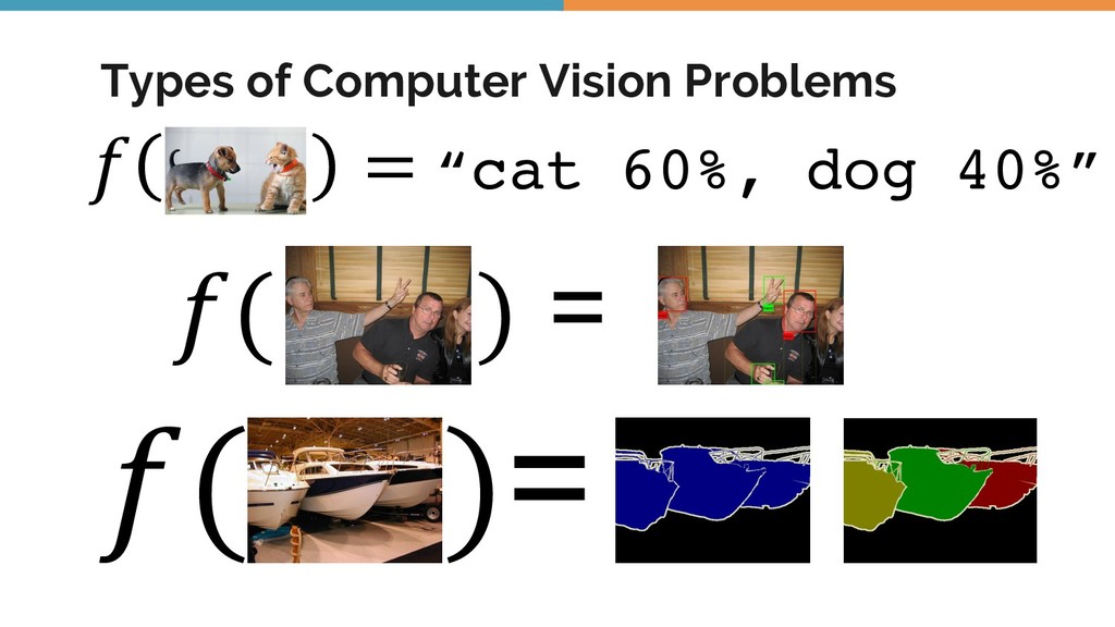
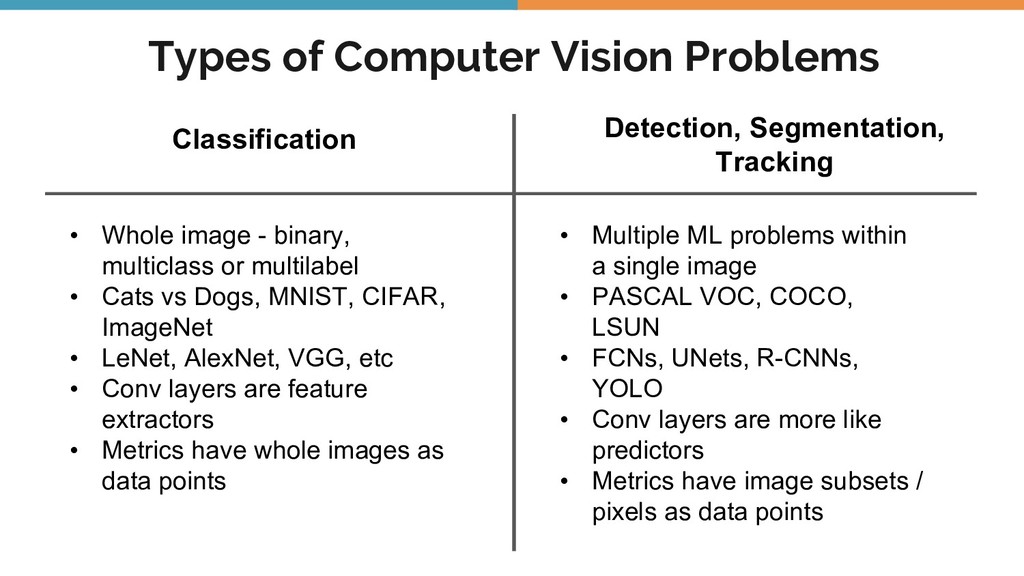
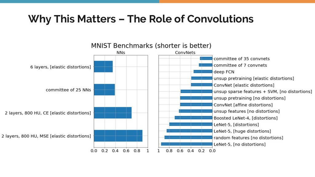
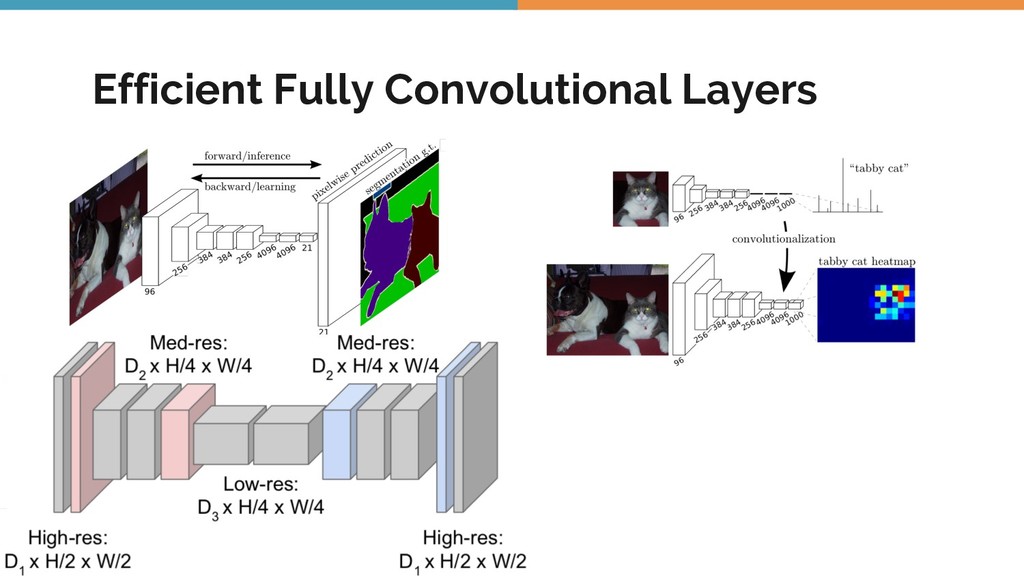
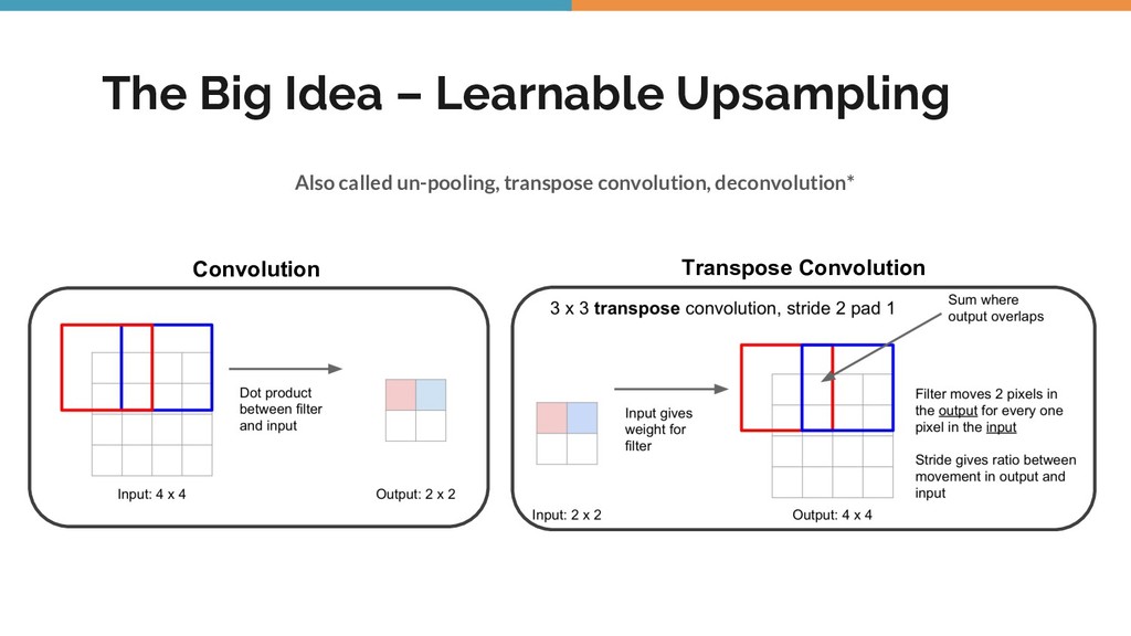
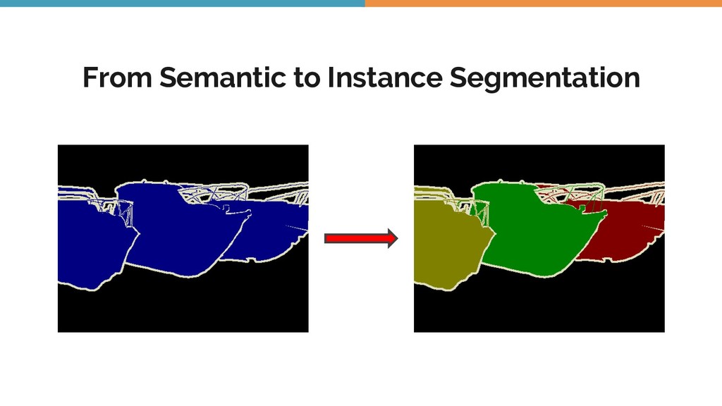
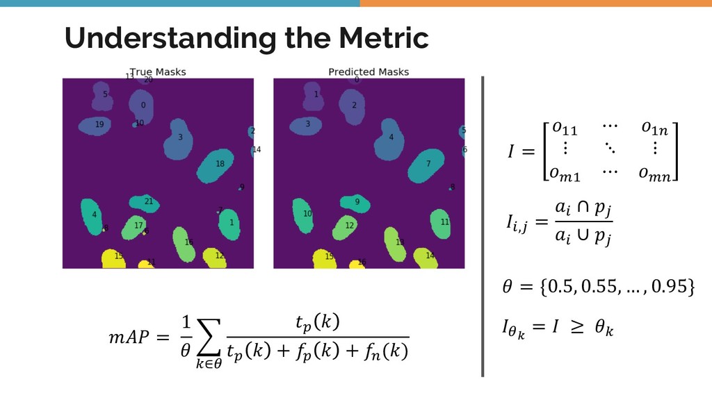
Object detection, tracking, semantic and instance segmentation are all staples of a computer vision system. This talk is an attempt to formalize the whole object detection problem from the ground up, with a focus on practical issues encountered when writing and deploying a deep learning model.

Proposal
--------

This talk is the result of my studies in the course of a couple of Kaggle competitions centered around segmentation. This was the first time I dealt with deep learning in a competitive setting. As I moved from sklearn to keras, the difference in how data is handled and models are trained was very noticeable. Beginning with the basics of object detection using simple image processing techniques, this talk will walk the audience through the practical intricacies of deep neural networks that perform object detection and classification. The talk focuses heavily on the data preprocessing, modeling and evaluation techniques rather than the theory, because of the latter there is no lack. As we see a spate of papers and preprints every day on deep learning and related techniques, being able to translate them into runnable Python code is becoming an increasingly useful skill.

This talk is _not_ about Kaggle itself. Success in such competitions depends on a lot more than simply the ability to write and train a good model - often, the difference between winning and losing is made by increasing the third or fourth decimal place. But, as Richard Hamming said in his lecture [**You and Your Research**](http://www.cs.virginia.edu/~robins/YouAndYourResearch.html),

> Great contributions are rarely done by adding another decimal place.

As I went from studying the classic textbooks in computer vision, before the days of deep learning, to the more contemporary and cutting edge work, I realized that I was producing ML models of a widely varying nature. Each of them had their pros and cons. Even though some of them performed relatively poorly on the evaluation data, they had other advantages like model simplicity, requiring less data and being faster to train.

This talk is all about navigating this entire landscape under different settings of data and computational resources.

Transcript

1. Practical Image Classification & Object Detection (or What I Wish I Knew Before Practicing Computer Vision) Jaidev Deshpande @jaidevd
2. Types of Computer Vision Problems ! = “cat 60%, dog 40%” !( ) = !( )= Source: ImageNet & PASCAL VOC Datasets
3. Types of Computer Vision Problems Classification Detection, Segmentation, Tracking • Whole image - binary, multiclass or multilabel • Cats vs Dogs, MNIST, CIFAR, ImageNet • LeNet, AlexNet, VGG, etc • Conv layers are feature extractors • Metrics have whole images as data points • Multiple ML problems within a single image • PASCAL VOC, COCO, LSUN • FCNs, UNets, R-CNNs, YOLO • Conv layers are more like predictors • Metrics have image subsets / pixels as data points
4. Why This Matters – The Role of Convolutions Source: http://yann.lecun.com/exdb/mnist/
5. ImageNet Benchmarks Source: “Deep Residual Learning”, He et. al, 2014
6. The Big Idea – Bayes Error Analysis Most time spent here ConvNets help here
7. Classification ConvNet Architectures LeNet Figure 2: An illustration of the architecture of our CNN, explicitly showing the delineation of responsibilities between the two GPUs. One GPU runs the layer-parts at the top of the figure while the other runs the layer-parts AlexNet
8. GoogLeNet* input Conv 7x7+2(S) MaxPool 3x3+2(S) LocalRespNorm Conv 1x1+1(V) Conv 3x3+1(S) LocalRespNorm MaxPool 3x3+2(S) Conv 1x1+1(S) Conv 1x1+1(S) Conv 1x1+1(S) MaxPool 3x3+1(S) DepthConcat Conv 3x3+1(S) Conv 5x5+1(S) Conv 1x1+1(S) Conv 1x1+1(S) Conv 1x1+1(S) Conv 1x1+1(S) MaxPool 3x3+1(S) DepthConcat Conv 3x3+1(S) Conv 5x5+1(S) Conv 1x1+1(S) MaxPool 3x3+2(S) Conv 1x1+1(S) Conv 1x1+1(S) Conv 1x1+1(S) MaxPool 3x3+1(S) DepthConcat Conv 3x3+1(S) Conv 5x5+1(S) Conv 1x1+1(S) Conv 1x1+1(S) Conv 1x1+1(S) Conv 1x1+1(S) MaxPool 3x3+1(S) AveragePool 5x5+3(V) DepthConcat Conv 3x3+1(S) Conv 5x5+1(S) Conv 1x1+1(S) Conv 1x1+1(S) Conv 1x1+1(S) Conv 1x1+1(S) MaxPool 3x3+1(S) DepthConcat Conv 3x3+1(S) Conv 5x5+1(S) Conv 1x1+1(S) Conv 1x1+1(S) Conv 1x1+1(S) Conv 1x1+1(S) MaxPool 3x3+1(S) DepthConcat Conv 3x3+1(S) Conv 5x5+1(S) Conv 1x1+1(S) Conv 1x1+1(S) Conv 1x1+1(S) Conv 1x1+1(S) MaxPool 3x3+1(S) AveragePool 5x5+3(V) DepthConcat Conv 3x3+1(S) Conv 5x5+1(S) Conv 1x1+1(S) MaxPool 3x3+2(S) Conv 1x1+1(S) Conv 1x1+1(S) Conv 1x1+1(S) MaxPool 3x3+1(S) DepthConcat Conv 3x3+1(S) Conv 5x5+1(S) Conv 1x1+1(S) Conv 1x1+1(S) Conv 1x1+1(S) Conv 1x1+1(S) MaxPool 3x3+1(S) DepthConcat Conv 3x3+1(S) Conv 5x5+1(S) Conv 1x1+1(S) AveragePool 7x7+1(V) FC Conv 1x1+1(S) FC FC SoftmaxActivation softmax0 Conv 1x1+1(S) FC FC SoftmaxActivation softmax1 SoftmaxActivation softmax2
9. Semantic Segmentation Semantic Segmentation Cow Grass Sky Trees Label each pixel in the image with a category label Don’t differentiate instances, only care about pixels This image is CC0 public domain Grass Cat Sky Trees Classify each pixel into a category.
10. Semantic Segmentation Architecture Semantic Segmentation Idea: Sliding Window Full image Extract patch Classify center pixel with CNN Cow Cow Grass
11. Semantic Segmentation – Fully Convolutional Networks Fei-Fei Li & Justin Johnson & Serena Yeung Lecture 11 - May 10, 2017 22 Semantic Segmentation Idea: Fully Convolutional Input: 3 x H x W Convolutions: D x H x W Conv Conv Conv Conv Scores: C x H x W argmax Predictions: H x W Design a network as a bunch of convolutional layers to make predictions for pixels all at once!
12. Efficient Fully Convolutional Layers an Shelhamer⇤ Trevor Darrell UC Berkeley er,trevor}@cs.berkeley.edu hat olu- els- en- al” uce and olu- nse We 22], olu- ons ne a om m a eg- ate- im- 96 384 256 4096 4096 21 21 backward/learning forward/inference pixelwise prediction segmentation g.t. 256 384 Figure 1. Fully convolutional networks can efficiently learn to make dense predictions for per-pixel tasks like semantic segmen- tation. We show that a fully convolutional network (FCN) trained end-to-end, pixels-to-pixels on semantic segmen- tation exceeds the state-of-the-art without further machin- ery. To our knowledge, this is the first work to train FCNs end-to-end (1) for pixelwise prediction and (2) from super- vised pre-training. Fully convolutional versions of existing networks predict dense outputs from arbitrary-sized inputs. Both learning and inference are performed whole-image-at-
13. The Big Idea – Learnable Upsampling Also called un-pooling, transpose convolution, deconvolution* ei-Fei Li & Justin Johnson & Serena Yeung Lecture 11 - May 10, 2017 33 Learnable Upsampling: Transpose Convolution Input: 4 x 4 Output: 2 x 2 Dot product between filter and input Filter moves 2 pixels in the input for every one pixel in the output Stride gives ratio between movement in input and output Recall: Normal 3 x 3 convolution, stride 2 pad 1 Fei-Fei Li & Justin Johnson & Serena Yeung Lecture 11 - May 10, 2017 36 Input: 2 x 2 Output: 4 x 4 Input gives weight for filter Sum where output overlaps Learnable Upsampling: Transpose Convolution 3 x 3 transpose convolution, stride 2 pad 1 Filter moves 2 pixels in the output for every one pixel in the input Stride gives ratio between movement in output and input Convolution Transpose Convolution
14. Putting it all together – the UNet
15. From Semantic to Instance Segmentation
16. Metric for Instance Segmentation – mAP of IoU Accuracy = 0.99 mAP of IoU = 0 Accuracy = 0.91 mAP of IoU = 0.7
17. Understanding the Metric ! = #$$ ⋯ #$& ⋮ ⋱ ⋮ #)$ ⋯ #)& !*,, = -* ∩ /, -* ∪ /, 1 = {0.5, 0.55, … , 0.95} !9: = ! ≥ 1< =>? = 1 1 A <∈9 CD E CD E + GD E + G& (E)
18. Learning Morphological Erosion* ! " = !$ " + !& ' exp − ,- " + ,. " . 20.
19. Hacking Keras Models >>> from keras.models import Sequential >>> from keras.layers import Dense >>> model = Sequential() >>> model.add(Dense(2, input_dim=1)) >>> model.add(Dense(1)) >>> from keras.models import Model >>> from keras.layers import Input >>> from keras.layers import Dense >>> visible = Input(shape=(2,)) >>> hidden = Dense(2)(visible) >>> model = Model(inputs=visible, ... outputs=hidden) Sequential API Functional API • Functional API is closer to the underlying computational graph • Do not ignore naming of layers • Useful callbacks: keras.callbacks.{History, ModelCheckpoint, EarlyStopping}
20. Gotchas with the Tensorflow Backend • A “batch” is always a set of images – getting pixelwise loss is not obvious. • Weighted classes and losses are allowed in Keras only at the batch level, not at the pixel level. • Pixelwise weights should be part of the computational graph - Functional API for the win! • Tensorflow losses expect logits, not activated outputs.
21. Make your life easy with • NumPy’s vectorization and array broadcasting (refer to @jakevdp’s excellent tutorial here. • Parallelization with joblib for preprocessing • Keras’ inbuilt image streaming and on-the-fly augmentation • Tensorboard
22. Acknowledgements • Aditi Dani for the endless typing of dictated code and slides, and enduring so many IPython kernel restarts. • Juxt SmartMandate Pvt Ltd for generously sponsoring my Coursera Deep Learning Specialization • Farhat Habib and Prabhu Ramachandran for their valuable inputs on everything SciPy.
23. Questions? • A verbose blog post on introducing pixelwise weighted losses into a UNet will be available soon • For link to slides, blog posts and other resources, watch https://twitter.com/jaidevd and #pydatadelhi