Scientific Visualization

Scientiﬁc Visualization May 22, 2014 ! PGI-1 / IAS-1 |
Scientiﬁc Visualization Workshop | Josef Heinen Member of the Helmholtz Association

May 22, 2014 Josef Heinen, Forschungszentrum Jülich, Peter Grünberg Institute,
Scientiﬁc IT Systems ✓ Motivation ✓ Scientiﬁc visualization software ✓ Visualization with Python ✓ Python performance optimizations ✓ Development tools ✓ Conclusion ✓ Future plans ✓ Discussion 2 Outline

Scientiﬁc IT Systems We need easy-to-use methods for: ✓ visualizing and analyzing two- and three- dimensional data sets, perhaps with a dynamic component ✓ creating publication-quality graphics ✓ making glossy ﬁgures for high impact journals or press releases 3 Motivation

Scientiﬁc IT Systems ✓ line / bar graphs, curve plots ✓ scatter plots ✓ surface plots, mesh rendering with iso-surface generation ✓ contour plots ✓ vector / streamline plots ✓ volume graphics ✓ molecule plots 4 Scientiﬁc plotting methods

Scientiﬁc IT Systems Scientiﬁc visualization tools ✓ Gnuplot ✓ Xmgrace ✓ OpenDX ✓ ParaView ✓ Mayavi2 ✓ MATLAB ✓ Mathematica ✓ Octave, Scilab, Freemat 5

Scientiﬁc IT Systems … drawbacks ✓ Gnuplot — limited functionality ✓ Xmgrace — too old, requires OSF/Motif (X11) ✓ OpenDX — no longer maintained (2007) ✓ ParaView — not very intuitive ✓ Mayavi2 — not very responsive ✓ MATLAB — 5 ﬂoating, 3 user licenses (16K €/year) ✓ Mathematica — expensive (~2.500 €/user) ✓ Octave, Scilab, Freemat — no syntax compatibility 6

Scientiﬁc IT Systems Scientiﬁc visualization APIs ✓ Matplotlib ✓ mlab, VTK ✓ OpenGL ✓ pgplot ✓ PyQtGraph ✓ PyQwt / PyQwt3D 7

Scientific IT Systems Scientific visualization APIs ✓ Matplotlib — de-facto standard (“workhorse”) ✓ mlab, VTK — versatile, but difficult to learn; slow ✓ OpenGL — large and complex ✓ pgplot — too old ✓ PyQtGraph — no yet mature ✓ PyQwt / PyQwt3D — currently unmaintained 8

Scientiﬁc IT Systems Remaining solutions GUI + API: ✓ ParaView ✓ Mayavi2 API: ✓ matplotlib ✓ n.n. ← Let’s talk about this later … 9 both based on VTK }

Scientiﬁc IT Systems 10 ParaView

Scientiﬁc IT Systems 11 Mayavi2

Scientiﬁc IT Systems 12 matplotlib

Scientiﬁc IT Systems Problems so far ✓ separated 2D and (hardware accelerated) 3D world ✓ some graphics backends "only" produce pictures   ➟ no presentation of continuous data streams ✓ bare minimum level of interoperability   ➟ limited user interaction ✓ poor performance on large data sets ✓ APIs are partly device- and platform-dependent 13

Scientiﬁc IT Systems Isn’t there an all-in-one solution? 14 All these components provide powerful APIs  for Python ! ! There must be a reason for that …

Scientiﬁc IT Systems … so let’s push for Python ✓ free and open ✓ dynamic typed language, easy to understand ✓ powerful modules for science, technology, engineering and mathematics (STEM): NumPy, SciPy, Pandas, SymPy ✓ great visualization libraries: Matplotlib, MayaVi, VTK, PyOpenGL ✓ techniques to boost execution speed: PyPy, Cython, PyOpenCL, PyCUDA, Numba ✓ wrapper for GUI toolkits: PyQt4, PyGTK, wxWidgets 15

Scientiﬁc IT Systems … get it up and running 16 IPython + NumPy + SciPy + Matplotlib  What else do we need?

Scientiﬁc IT Systems … achieve more Python performance Numba: compiles annotated Python and NumPy code to LLVM (through decorators) ✓ just-in-time compilation ✓ vectorization ✓ parallelization NumbaPro: adds support for multicore and GPU architectures 17 (* Numba (Pro) is part of Anaconda (Accelerate), a (commercial) Python distribution from Continuum Analytics

Scientiﬁc IT Systems … achieve more graphics performance and interop GR framework: a universal framework for cross- platform visualization (* ✓ procedural graphics backend  ➟ presentation of continuous data streams ✓ coexistent 2D and 3D world ✓ interoperability with GUI toolkits  ➟ good user interaction 18 (* The GR framework is an in-house project initiated by the group Scientiﬁc IT Systems

Scientiﬁc IT Systems “Our” Scientiﬁc Python distribution 19 IPython + NumPy + SciPy + Numba + GR framework + PyOpenGL + PyOpenCL + PyCUDA + PyQt4/PyGTK/wxWidgets    ➟ more performance and interoperability

Scientiﬁc IT Systems How can we use it? ✓ GR framework (and other mentioned packages) available on all Linux and OS X machines  (Python and IPython) at PGI / JCNS:  % gr  % igr" ✓ GR framework can also be used with Anaconda:  % anaconda ✓ Windows version(s) on request 20

Scientiﬁc IT Systems Batteries included ✓ NumPy — package for numerical computation ✓ SciPy — collection of numerical algorithms and speciﬁc toolboxes ✓ Matplotlib — popular plotting package ✓ Pandas — provides high-performance, easy to use data structures ✓ SymPy — symbolic mathematics and computer algebra ✓ IPython — rich interactive interface (including IPython notebook) ✓ Mayavi2 — 3D visualization framework, based on VTK ✓ scikit-image — algorithms for image processing ✓ h5py, PyTables — managing hierarchical datasets (HDF5) 21

Scientific IT Systems Visualization with Python 22 GKS logical device drivers C / C++ GKS GR OpenGL (WGL / CGL / GLX) POV-Ray  generation off-screen rendering direct rendering Browser JavaScript  generation WebGL IPython / PyPy/ Anaconda Win32 X11 GKSTerm gksqt Java gksweb Qt Quartz PDF C / ObjC OpenGL ES glgr / iGR App socket  communication Qt / wx  event loop 0MQ OpenGL More logical device drivers / plugins: – CGM, GKSM, GIF, RF, UIL – WMF, Xfig – GS (BMP, JPEG, PNG, TIFF) ... HTML5 wx POV-Ray GLUT wxGLCanvas QGLWidget ... SVG PS MOV GR3 Highlights: – simultaneous output to multiple output devices – direct generation of MPEG4 image sequences – flicker-free display ("double buffering")

Scientiﬁc IT Systems Presentation of continuous data streams in 2D ... 23 from numpy import sin, cos, sqrt, pi, array import gr ! def rk4(x, h, y, f): k1 = h * f(x, y) k2 = h * f(x + 0.5 * h, y + 0.5 * k1) k3 = h * f(x + 0.5 * h, y + 0.5 * k2) k4 = h * f(x + h, y + k3) return x + h, y + (k1 + 2 * (k2 + k3) + k4) / 6.0 ! def damped_pendulum_deriv(t, state): theta, omega = state return array([omega, -gamma * omega - 9.81 / L * sin(theta)]) ! def pendulum(t, theta, omega) gr.clearws() ... # draw pendulum (pivot point, rod, bob, ...) gr.updatews() ! theta = 70.0 # initial angle gamma = 0.1 # damping coefficient L = 1 # pendulum length t = 0 dt = 0.04 state = array([theta * pi / 180, 0]) ! while t < 30: t, state = rk4(t, dt, state, damped_pendulum_deriv) theta, omega = state pendulum(t, theta, omega)

Scientiﬁc IT Systems ... with full 3D functionality 24 from numpy import sin, cos, array import gr, gr3 ! def rk4(x, h, y, f): k1 = h * f(x, y) k2 = h * f(x + 0.5 * h, y + 0.5 * k1) k3 = h * f(x + 0.5 * h, y + 0.5 * k2) k4 = h * f(x + h, y + k3) return x + h, y + (k1 + 2 * (k2 + k3) + k4) / 6.0 ! def pendulum_derivs(t, state): t1, w1, t2, w2 = state a = (m1 + m2) * l1 b = m2 * l2 * cos(t1 - t2) c = m2 * l1 * cos(t1 - t2) d = m2 * l2 e = -m2 * l2 * w2**2 * sin(t1 - t2) - 9.81 * (m1 + m2) * sin(t1) f = m2 * l1 * w1**2 * sin(t1 - t2) - m2 * 9.81 * sin(t2) return array([w1, (e*d-b*f) / (a*d-c*b), w2, (a*f-c*e) / (a*d-c*b)]) ! def double_pendulum(theta, length, mass): gr.clearws() gr3.clear() ! ... # draw pivot point, rods, bobs (using 3D meshes) ! gr3.drawimage(0, 1, 0, 1, 500, 500, gr3.GR3_Drawable.GR3_DRAWABLE_GKS) gr.updatews()

Scientiﬁc IT Systems ... in real-time 25 import wave, pyaudio import numpy import gr ! SAMPLES=1024 FS=44100 # Sampling frequency ! f = [FS/float(SAMPLES)*t for t in range(1, SAMPLES/2+1)] ! wf = wave.open('Monty_Python.wav', 'rb') pa = pyaudio.PyAudio() stream = pa.open(format=pa.get_format_from_width(wf.getsampwidth()), channels=wf.getnchannels(), rate=wf.getframerate(), output=True) ! ... ! data = wf.readframes(SAMPLES) while data != '' and len(data) == SAMPLES * wf.getsampwidth(): stream.write(data) amplitudes = numpy.fromstring(data, dtype=numpy.short) power = abs(numpy.fft.fft(amplitudes / 65536.0))[:SAMPLES/2] ! gr.clearws() ... gr.polyline(SAMPLES/2, f, power) gr.updatews() data = wf.readframes(SAMPLES)

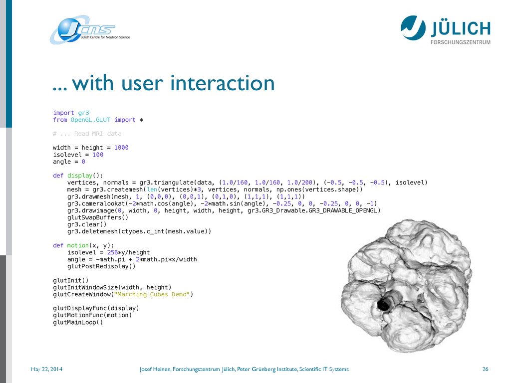
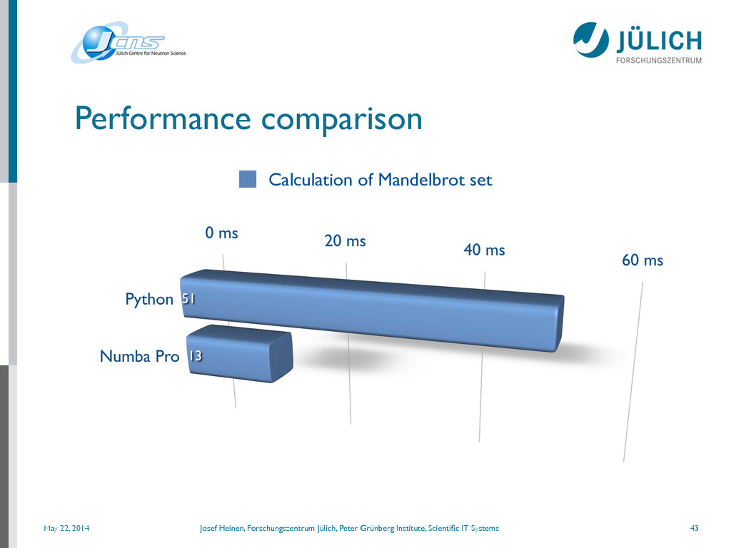
Scientiﬁc IT Systems ... with user interaction 26 import gr3 from OpenGL.GLUT import * # ... Read MRI data  width = height = 1000 isolevel = 100 angle = 0 ! def display(): vertices, normals = gr3.triangulate(data, (1.0/160, 1.0/160, 1.0/200), (-0.5, -0.5, -0.5), isolevel) mesh = gr3.createmesh(len(vertices)*3, vertices, normals, np.ones(vertices.shape)) gr3.drawmesh(mesh, 1, (0,0,0), (0,0,1), (0,1,0), (1,1,1), (1,1,1)) gr3.cameralookat(-2*math.cos(angle), -2*math.sin(angle), -0.25, 0, 0, -0.25, 0, 0, -1) gr3.drawimage(0, width, 0, height, width, height, gr3.GR3_Drawable.GR3_DRAWABLE_OPENGL) glutSwapBuffers() gr3.clear() gr3.deletemesh(ctypes.c_int(mesh.value)) def motion(x, y): isolevel = 256*y/height angle = -math.pi + 2*math.pi*x/width glutPostRedisplay() glutInit() glutInitWindowSize(width, height) glutCreateWindow("Marching Cubes Demo") ! glutDisplayFunc(display) glutMotionFunc(motion) glutMainLoop()

Scientiﬁc IT Systems ... with Qt 27

Scientiﬁc IT Systems ... and wxWidgets 28

Scientiﬁc IT Systems Scalable graphics in Web browsers 29

Scientiﬁc IT Systems Import PDF 30 import gr (w, h, data) = gr.readimage("fs.pdf") if w < h: r = float(w)/h gr.setviewport(0.5*(1-r), 0.5*(1+r), 0, 1); else: r = float(h)/w gr.setviewport(0, 1, 0.5*(1-r), 0.5*(1+r)); gr.drawimage(0, 1, 0, 1, w, h, data) gr.updatews()

Scientiﬁc IT Systems Success stories (I) 31 World’s most powerful laboratory small-angle X-ray scattering facility at Forschungszentrum Jülich

Scientiﬁc IT Systems Success stories (II) 32 BornAgain A software to simulate and ﬁt neutron and x-ray scattering at grazing incidence (GISANS and GISAXS), using distorted- wave Born approximation (DWBA) Nframes = 100 radius = 1 height = 4 distance = 5 ! def RunSimulation(): # defining materials mAir = HomogeneousMaterial("Air", 0.0, 0.0) mSubstrate = HomogeneousMaterial("Substrate", 6e-6, 2e-8) mParticle = HomogeneousMaterial("Particle", 6e-4, 2e-8) # collection of particles cylinder_ff = FormFactorCylinder(radius, height) cylinder = Particle(mParticle, cylinder_ff) particle_layout = ParticleLayout() particle_layout.addParticle(cylinder) # interference function interference = InterferenceFunction1DParaCrystal(distance, 3 * nanometer) particle_layout.addInterferenceFunction(interference) # air layer with particles and substrate form multi layer air_layer = Layer(mAir) air_layer.setLayout(particle_layout) substrate_layer = Layer(mSubstrate) multi_layer = MultiLayer() multi_layer.addLayer(air_layer) multi_layer.addLayer(substrate_layer) # build and run experiment simulation = Simulation() simulation.setDetectorParameters(250, -4*degree, 4*degree, 250, 0*degree, 8*degree) simulation.setBeamParameters(1.0 * angstrom, 0.2 * degree, 0.0 * degree) simulation.setSample(multi_layer) simulation.runSimulation() return simulation.getIntensityData().getArray() def SetParameters(i): radius = (1. + (3.0/Nframes)*i) * nanometer height = (1. + (4.0/Nframes)*i) * nanometer distance = (10. - (1.0/Nframes)*i) * nanometer ! for i in range(100): SetParameters(i) result = RunSimulation() gr.pygr.imshow(numpy.log10(numpy.rot90(result, 1)), cmap=gr.COLORMAP_PILATUS)

Scientiﬁc IT Systems Success stories (III) 33 NICOS a network-based control system written for neutron scattering instruments at the FRM II

Scientiﬁc IT Systems Coming soon:  Python moldyn package … 34

Scientiﬁc IT Systems … with video output 35

Scientiﬁc IT Systems … and POV-Ray output 36

Scientiﬁc IT Systems … in highest resolution 37

Scientiﬁc IT Systems Performance optimizations ✓ NumPy  module for handling multi-dimensional arrays (ndarray) ✓ Numba (Anaconda) ✓ just-in-time compilation driven by @autojit- or @jit- decorators (LLVM) ✓ vectorization of ndarray based functions (ufuncs) ✓ Numba Pro (Anaconda Accelerate) ✓ parallel loops and ufuncs ✓ execution of ufunfs on GPUs ✓ “Python” GPU kernels ✓ GPU optimized libraries (cuBLAS, cuFFT, cuRAND) 38

Scientiﬁc IT Systems Realization ✓ NumPy  vector operations on ndarrays instead of loops  ➟ works in any NumPy Python environment ✓ Numba (Anaconda)  add @jit and @autojit decorators  ➟ useful for “many” function calls with “big” arrays ✓ Numba Pro (Anaconda Accelerate)  add @vectorize decorators  implementation of multi-core / GPU kernels in "Python"   switch to GPU-optimized features  ➟ useful only for "large" arrays  performance 39

Scientiﬁc IT Systems Particle simulation 40 import numpy as np ! ! N = 300 # number of particles M = 0.05 * np.ones(N) # masses size = 0.04 # particle size ! ! def step(dt, size, a): a[0] += dt * a[1] # update positions ! n = a.shape[1] D = np.empty((n, n), dtype=np.float) for i in range(n): for j in range(n): dx = a[0, i, 0] - a[0, j, 0] dy = a[0, i, 1] - a[0, j, 1] D[i, j] = np.sqrt(dx*dx + dy*dy) ! ... # find pairs of particles undergoing a collision ... # check for crossing boundary return a ... ! a[0, :] = -0.5 + np.random.random((N, 2)) # positions a[1, :] = -0.5 + np.random.random((N, 2)) # velocities a[0, :] *= (4 - 2*size) dt = 1. / 30 ! while True: a = step(dt, size, a) .... ! from numba.decorators import autojit ! ! ! ! ! @autojit ! ! ! ! ! ! ! ! ! ! ! ! ! ! ! ! ! ! ! ! ! ! !

Scientiﬁc IT Systems Diffusion 41 import numpy ! ! dx = 0.005 dy = 0.005 a = 0.5 dt = dx*dx*dy*dy/(2*a*(dx*dx+dy*dy)) timesteps = 300 ! nx = int(1/dx) ny = int(1/dy) ui = numpy.zeros([nx,ny]) u = numpy.zeros([nx,ny]) ! ! def diff_step(u, ui): for i in range(1,nx-1): for j in range(1,ny-1): uxx = ( ui[i+1,j] - 2*ui[i,j] + ui[i-1, j] )/(dx*dx) uyy = ( ui[i,j+1] - 2*ui[i,j] + ui[i, j-1] )/(dy*dy) u[i,j] = ui[i,j]+dt*a*(uxx+uyy) ! ! ! for m in range(timesteps): diff_step (u, ui) ui = numpy.copy(u) ... ! from numba.decorators import jit ! ! ! ! ! ! ! ! ! ! ! ! ! ! ! ! ! ! ! ! diff_step_numba = jit('void(f8[:,:], f8[:,:])')(diff_step) ! ! diff_step_numba(u, ui) !

Scientiﬁc IT Systems Mandelbrot set 42 from numbapro import vectorize import numpy as np ! @vectorize(['uint8(uint32, f8, f8, f8, f8, uint32, uint32, uint32)'], target='gpu') def mandel(tid, min_x, max_x, min_y, max_y, width, height, iters): pixel_size_x = (max_x - min_x) / width pixel_size_y = (max_y - min_y) / height ! x = tid % width y = tid / width ! real = min_x + x * pixel_size_x imag = min_y + y * pixel_size_y ! c = complex(real, imag) z = 0.0j ! for i in range(iters): z = z * z + c if (z.real * z.real + z.imag * z.imag) >= 4: return i ! return 255 ! ! def create_fractal(min_x, max_x, min_y, max_y, width, height, iters): tids = np.arange(width * height, dtype=np.uint32) return mandel(tids, np.float64(min_x), np.float64(max_x), np.float64(min_y), np.float64(max_y), np.uint32(height), np.uint32(width), np.uint32(iters))

Scientiﬁc IT Systems Performance comparison 43 Calculation of Mandelbrot set

Scientiﬁc IT Systems Numba (Pro) review 44 ✓ functions with numerical code can be compiled with little effort and lead to impressive results ✓ numerical code should be separated from logic statements (and processing of lists, dictionaries) ✓ advanced Technologie due to LLVM intermediate language (LLVM IR) ✓ easy installation and maintenance  Download link (Continuum Analytics): http://www.continuum.io/downloads % bash Anaconda-1.x.x-[Linux|MacOSX]-x86[_64].sh % conda update conda % conda update anaconda

Scientiﬁc IT Systems Development tools 45 You can use your favorite editor and start Python in a shell. But  the impatient user should chose a development environment:

Scientiﬁc IT Systems IPython console 46

Scientiﬁc IT Systems IPython notebook 47

Scientiﬁc IT Systems Spyder 48

Scientiﬁc IT Systems PyCharm 49

Scientiﬁc IT Systems Bokeh 50 import numpy as np from scipy.integrate import odeint from bokeh.plotting import * ! sigma = 10 rho = 28 beta = 8.0/3 theta = 3 * np.pi / 4 ! def lorenz(xyz, t): x, y, z = xyz x_dot = sigma * (y - x) y_dot = x * rho - x * z - y z_dot = x * y - beta* z return [x_dot, y_dot, z_dot] ! initial = (-10, -7, 35) t = np.arange(0, 100, 0.006) ! solution = odeint(lorenz, initial, t) ! x = solution[:, 0] y = solution[:, 1] z = solution[:, 2] xprime = np.cos(theta) * x - np.sin(theta) * y ! colors = ["#C6DBEF", "#9ECAE1", "#6BAED6", “#4292C6", "#2171B5", "#08519C", "#08306B",] ! output_file("lorenz.html", title="lorenz.py example") ! multi_line(np.array_split(xprime, 7), np.array_split(z, 7), line_color=colors, line_alpha=0.8, line_width=1.5, tools=“pan,wheel_zoom,box_zoom,reset,previewsave", title="lorenz example", name="lorenz_example") ! show() # open a browser

Scientiﬁc IT Systems Resources ✓ Website: http://gr-framework.org ✓ PyPI: https://pypi.python.org/pypi/gr ✓ Git Repository: http://github.com/jheinen/gr ✓ Binstar: https://binstar.org/jheinen/gr ✓ Talk: Scientiﬁc Visualization Workshop (PDF, HTML) 51

Scientiﬁc IT Systems Website 52

Scientiﬁc IT Systems Git-Repo 53

Scientiﬁc IT Systems PyPI 54

Scientiﬁc IT Systems Binstar 55

Scientiﬁc IT Systems Conclusion ✓ The use of Python with the GR framework and Numba (Pro) extensions allows the realization of high-performance visualization applications in scientiﬁc and technical environments ✓ The GR framework can seamlessly be integrated into "foreign" Python environments, e.g. Anaconda, by using the ctypes mechanism ✓ Anaconda (Accelerate) is an easy to manage (commercial) Python distribution that can be enhanced by the use of the GR framework with its functions for real-time or 3D visualization applications 56

Scientiﬁc IT Systems Future plans ✓ implement your(!) feature requests ✓ moldyn package for Python ✓ more ✓ tutorials ✓ convenience functions ✓ documentation ✓ examples (gallery) ✓ IPython notebook integration ✓ Bokeh integration 57

Scientiﬁc IT Systems Thank you for your attention References: Numba, A Dynamic Python compiler for Science: http://lanyrd.com/2013/pycon/scdyzh  Continuum Analytics: http://www.continuum.io ! Contact: [email protected]  @josef_heinen" ! Thanks to: Florian Rhiem, Ingo Heimbach, Christian Felder, David Knodt, Jörg Winkler, Fabian Beule,  Marcel Dück, Marvin Goblet, et al. 58

Scientific Visualization

Scientific Visualization

More Decks by Josef Heinen

Other Decks in Programming

Featured

Transcript