Affymetrix Microarray Tutorial

Tutorial covering the basics of an Affymetrix microarray experiment, using data obtained from a GEO experiment.

Transcript

1. Cleaning and Analyzing Microarray Raw Data for WGCNA For use by the DHG Lab Jillian Haney 08/12/15
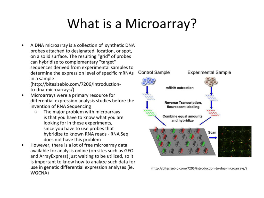
2. What is a Microarray? • A DNA microarray is a collection of synthetic DNA probes attached to designated location, or spot, on a solid surface. The resulting "grid" of probes can hybridize to complementary "target" sequences derived from experimental samples to determine the expression level of specific mRNAs in a sample (http://bitesizebio.com/7206/introduction- to-dna-microarrays/) • Microarrays were a primary resource for differential expression analysis studies before the invention of RNA Sequencing ◦ The major problem with microarrays is that you have to know what you are looking for in these experiments, since you have to use probes that hybridize to known RNA reads - RNA Seq does not have this problem • However, there is a lot of free microarray data available for analysis online (on sites such as GEO and ArrayExpress) just waiting to be utilized, so it is important to know how to analyze such data for use in genetic differential expression analyses (ie. WGCNA) (http://bitesizebio.com/7206/introduction-to-dna-microarrays/)
3. How Do We Perform Microarray Analysis? • R Statistical Programming – R is used to process the massive amounts of data acquired from microarray studies – This is the most efficient language in which to perform statistical analysis with microarray data • Helpful Introduction to R – http://rafalab.jhsph.edu/688/labs/lab1.pdf
4. Important Notes • Although most of the steps in this tutorial are needed for every microarray analysis (steps 8 and 9 are sometimes not required, if the data is given in terms of genes instead of probes), many of the specific instructions and code examples in this tutorial are geared towards affymetrix microarrays • For other platforms (illumina, nimblegen, etc.) you may need to find the relevant R commands to complete each step on your own – Google is an excellent resource for this! • Refer to the ‘Cleaning and Analyzing Raw Microarray Data for WGCNA’ document for specific code examples and more detailed explanations for all steps
5. Overview 1. Get Data 2. QC on Non-Normalized Data 3. Normalization 4. Batch Correction 5. Outlier Removal 6. QC on Normalized Data 7. Covariate Analysis 8. Annotating Probes 9. Collapse Rows 10. Differential Expression Analysis
6. 1. Get Data • Find the microarray data that you want to analyze – http://www.ncbi.nlm.nih.gov/geo/ – https://www.ebi.ac.uk/arrayexpress/ – Use a computer program such as 7-Zip to save microarray data as ‘.CEL’ files in a folder on your computer (for relevant microarrays, ie. affymetrix) • Create a datMeta excel spreadsheet with phenotypic data using obtained microarray data • For affymetrix arrays, Use “ReadAffy” function to extract – expression matrix (exprs) – phenotypic data (pData) – protocolData
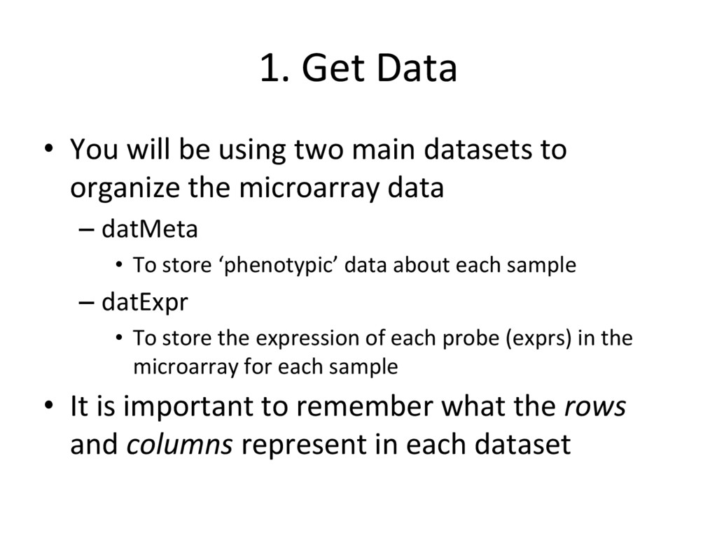
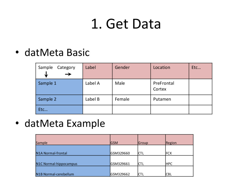
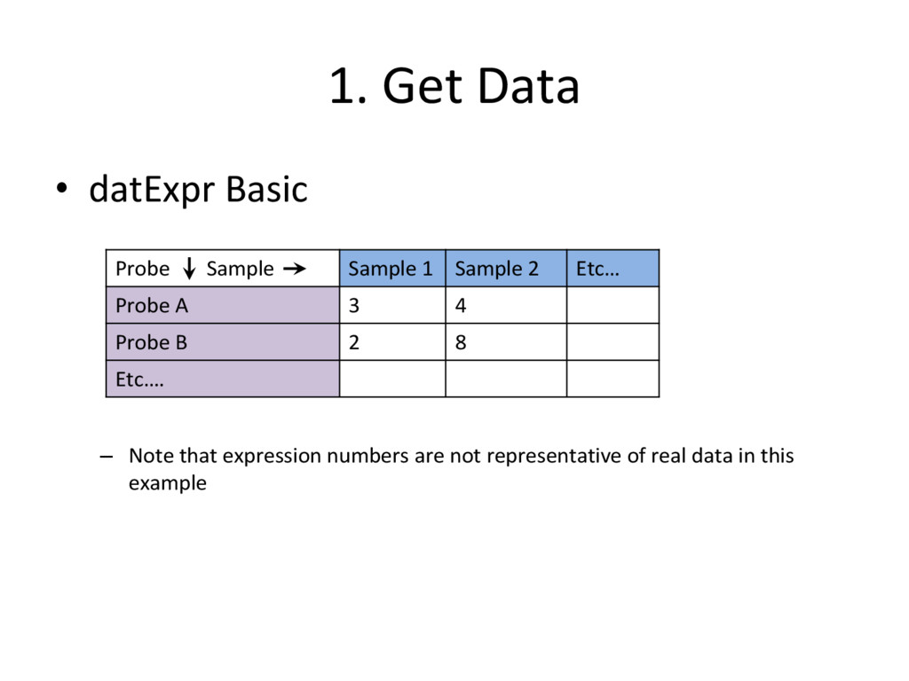
7. 1. Get Data • You will be using two main datasets to organize the microarray data – datMeta • To store ‘phenotypic’ data about each sample – datExpr • To store the expression of each probe (exprs) in the microarray for each sample • It is important to remember what the rows and columns represent in each dataset
8. 1. Get Data • datMeta Basic • datMeta Example Sample Category Label Gender Location Etc… Sample 1 Label A Male PreFrontal Cortex Sample 2 Label B Female Putamen Etc… Sample GSM Group Region N1A Normal-frontal GSM329660 CTL FCX N1C Normal-hippocampus GSM329661 CTL HPC N1B Normal-cerebellum GSM329662 CTL CBL
9. 1. Get Data • datExpr Basic – Note that expression numbers are not representative of real data in this example Probe Sample Sample 1 Sample 2 Etc… Probe A 3 4 Probe B 2 8 Etc….
10. Overview 1. Get Data 2. QC on Non-Normalized Data 3. Normalization 4. Batch Correction 5. Outlier Removal 6. QC on Normalized Data 7. Covariate Analysis 8. Annotating Probes 9. Collapse Rows 10. Differential Expression Analysis
11. 2. QC on Non-Normalized Data • Before normalizing the data, we want to make sure that our raw data looks normal • QC = Quality Control • We perform three basic tests – Boxplot – Histogram – MDS
12. 2. QC on Non-Normalized Data • Boxplot: gives us an idea of how much each sample is expressed – x-axis: samples (red are PD, black are control) – y-axis: intensity of each sample
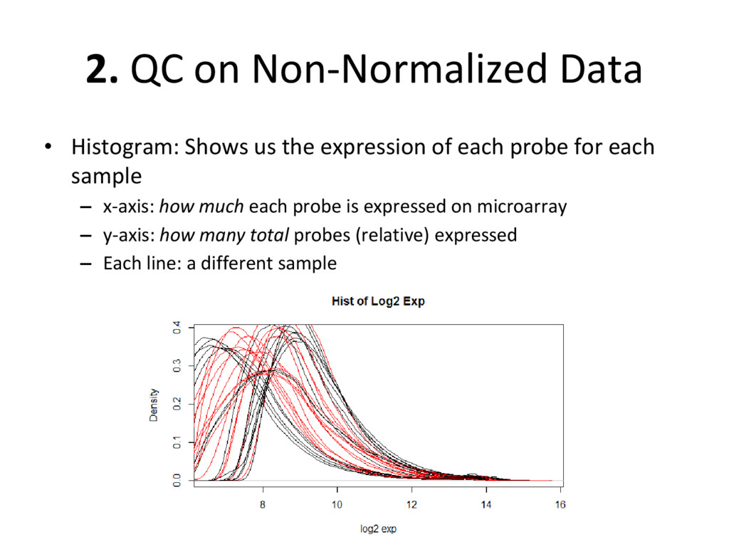
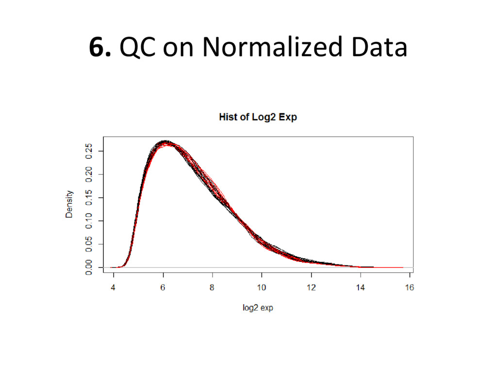
13. 2. QC on Non-Normalized Data • Histogram: Shows us the expression of each probe for each sample – x-axis: how much each probe is expressed on microarray – y-axis: how many total probes (relative) expressed – Each line: a different sample
14. 2. QC on Non-Normalized Data • MDS (Multi-Dimensional Scaling) Plot – Visual representation of how similar samples are in their expression using principal component analysis (PCA)
15. Overview 1. Get Data 2. QC on Non-Normalized Data 3. Normalization 4. Batch Correction 5. Outlier Removal 6. QC on Normalized Data 7. Covariate Analysis 8. Annotating Probes 9. Collapse Rows 10. Differential Expression Analysis
16. 3. Normalization • Normalization helps to remove experimental error • RMA (robust multi-array) Normalization for affymetrix arrays – Background Correction (some probes bind to nothing/eliminate background noise) – Probe Summarization – Quantile Normalization (log2 transformation)
17. Overview 1. Get Data 2. QC on Non-Normalized Data 3. Normalization 4. Batch Correction 5. Outlier Removal 6. QC on Normalized Data 7. Covariate Analysis 8. Annotating Probes 9. Collapse Rows 10. Differential Expression Analysis
18. 4. Batch Correction • We want to remove singular batches, since we cannot accurately account for the error introduced in those batches 1. Get Batch 2. Correct Batch
19. Overview 1. Get Data 2. QC on Non-Normalized Data 3. Normalization 4. Batch Correction 5. Outlier Removal 6. QC on Normalized Data 7. Covariate Analysis 8. Annotating Probes 9. Collapse Rows 10. Differential Expression Analysis
20. 5. Outlier Removal • Outliers in the data introduce variance that decreases the accuracy of our final data analysis • We identify these outliers with network connectivity based statistics, and then remove these outliers from the data
21. Overview 1. Get Data 2. QC on Non-Normalized Data 3. Normalization 4. Batch Correction 5. Outlier Removal 6. QC on Normalized Data 7. Covariate Analysis 8. Annotating Probes 9. Collapse Rows 10. Differential Expression Analysis
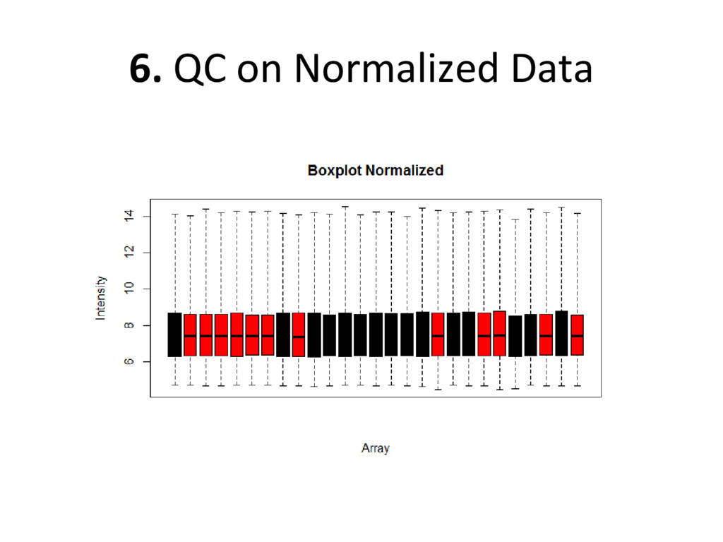
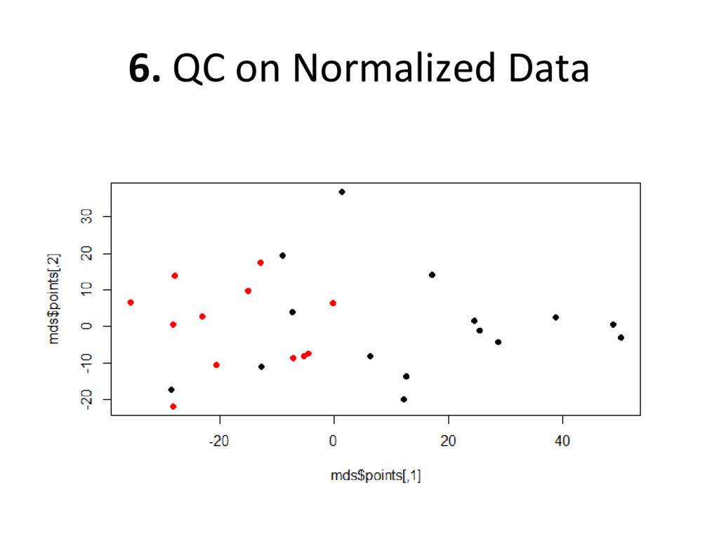
22. 6. QC on Normalized Data • We perform another QC on normalized, batch corrected, and outlier removed data to see if we have accurately removed experimental error – Box plot: are the medians/means of the data about the same? – Histogram: do the lines overlap more strongly than before? – MDS plot: do control and diseased samples separate more from each other? • If you answered ‘yes’ to each of these, you have correctly removed error from your data
23. 6. QC on Normalized Data
24. 6. QC on Normalized Data
25. 6. QC on Normalized Data
26. Overview 1. Get Data 2. QC on Non-Normalized Data 3. Normalization 4. Batch Correction 5. Outlier Removal 6. QC on Normalized Data 7. Covariate Analysis 8. Annotating Probes 9. Collapse Rows 10. Differential Expression Analysis
27. 7. Covariate Analysis • It’s important that all biological and technical covariates are not confounded by group/disease state • We don’t want the other factors to be correlated • We want the p-value between disease state and factors such as age, gender, etc. to be greater than 0.05 • If this is not the case for one of your factors, then you need to remove the outlier data points within the problem factor from your data-set, as they introduce confounding error that is not controlled for in the experiment
28. Overview 1. Get Data 2. QC on Non-Normalized Data 3. Normalization 4. Batch Correction 5. Outlier Removal 6. QC on Normalized Data 7. Covariate Analysis 8. Annotating Probes 9. Collapse Rows 10. Differential Expression Analysis
29. 8. Annotating Probes • Now we have our clean data, but we still need to determine which genes our microarray probes tagged, and then align this ‘geneDat’ with our ‘datExpr’ • We use bioMart to re-annotate probes with ensembl gene IDs based on the most recent species genome knowledge • Be sure that your geneDat and datExpr have the same probes in the same order before making the rownames of datExpr your gene IDs
30. Overview 1. Get Data 2. QC on Non-Normalized Data 3. Normalization 4. Batch Correction 5. Outlier Removal 6. QC on Normalized Data 7. Covariate Analysis 8. Annotating Probes 9. Collapse Rows 10. Differential Expression Analysis
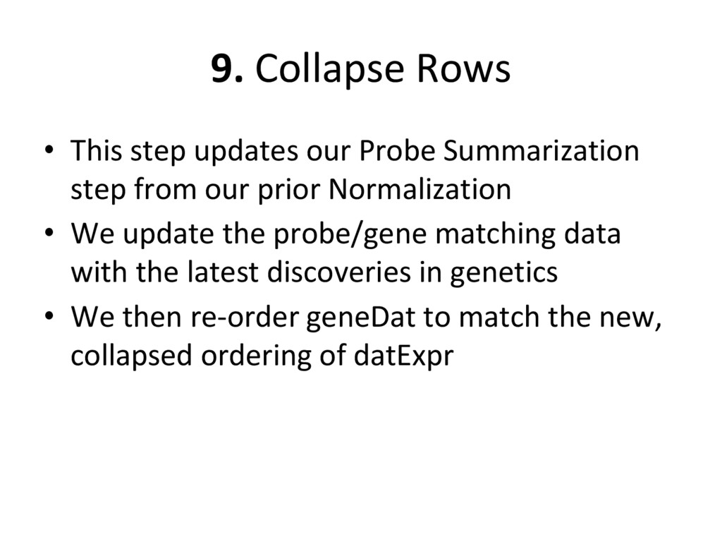
31. 9. Collapse Rows • This step updates our Probe Summarization step from our prior Normalization • We update the probe/gene matching data with the latest discoveries in genetics • We then re-order geneDat to match the new, collapsed ordering of datExpr
32. Overview 1. Get Data 2. QC on Non-Normalized Data 3. Normalization 4. Batch Correction 5. Outlier Removal 6. QC on Normalized Data 7. Covariate Analysis 8. Annotating Probes 9. Collapse Rows 10. Differential Expression Analysis
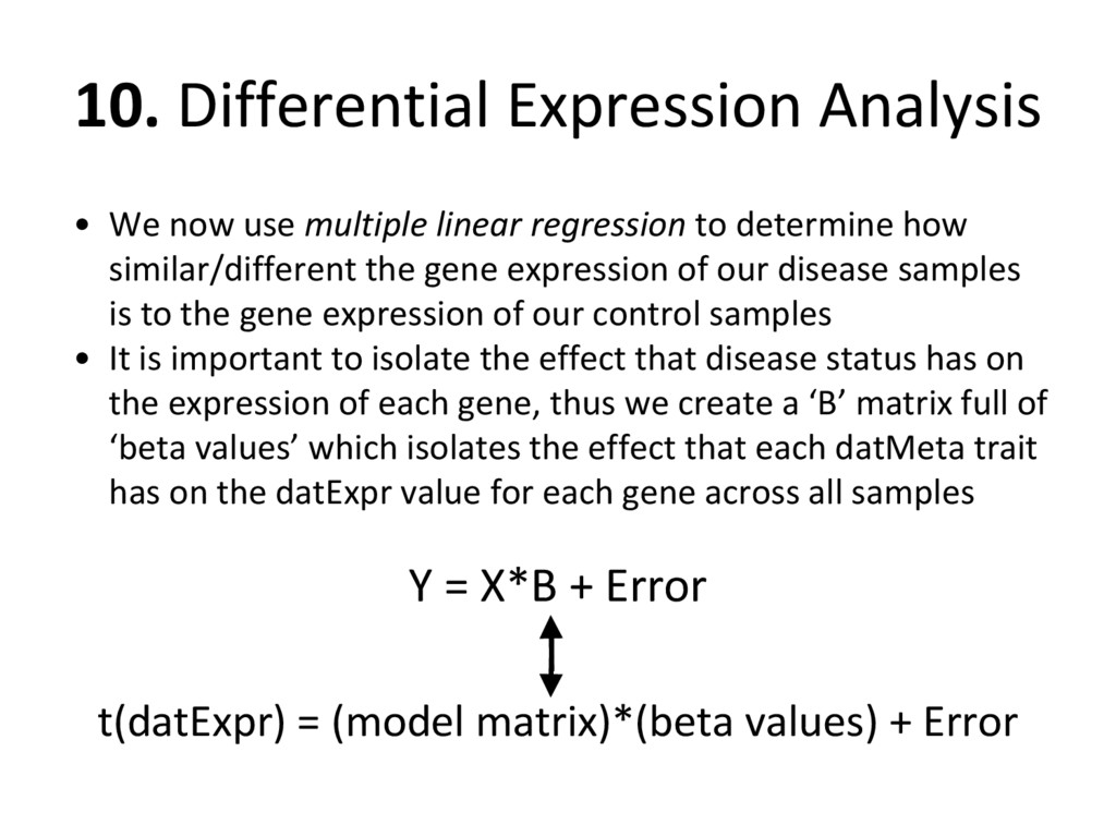
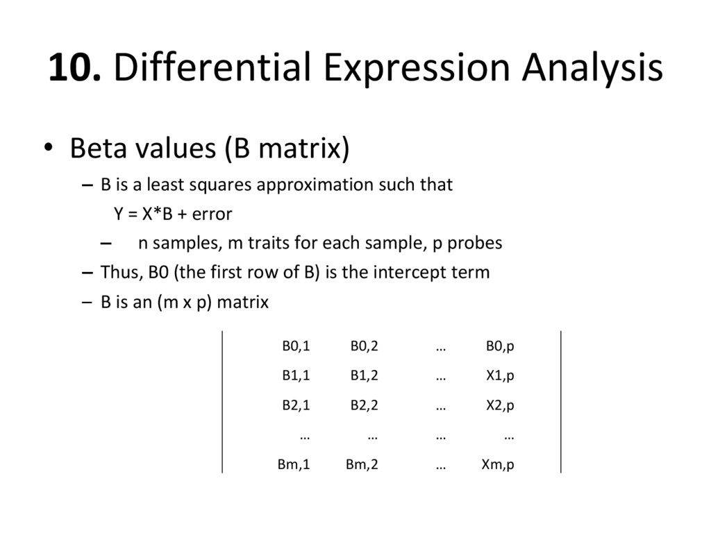
33. 10. Differential Expression Analysis • We now use multiple linear regression to determine how similar/different the gene expression of our disease samples is to the gene expression of our control samples • It is important to isolate the effect that disease status has on the expression of each gene, thus we create a ‘B’ matrix full of ‘beta values’ which isolates the effect that each datMeta trait has on the datExpr value for each gene across all samples Y = X*B + Error t(datExpr) = (model matrix)*(beta values) + Error
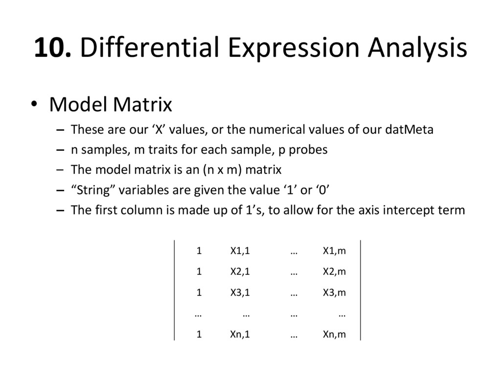
34. 10. Differential Expression Analysis • Model Matrix – These are our ‘X’ values, or the numerical values of our datMeta – n samples, m traits for each sample, p probes – The model matrix is an (n x m) matrix – “String” variables are given the value ‘1’ or ‘0’ – The first column is made up of 1’s, to allow for the axis intercept term 1 X1,1 … X1,m 1 X2,1 … X2,m 1 X3,1 … X3,m … … … … 1 Xn,1 … Xn,m
35. 10. Differential Expression Analysis • Beta values (B matrix) – B is a least squares approximation such that Y = X*B + error – n samples, m traits for each sample, p probes – Thus, B0 (the first row of B) is the intercept term – B is an (m x p) matrix B0,1 B0,2 … B0,p B1,1 B1,2 … X1,p B2,1 B2,2 … X2,p … … … … Bm,1 Bm,2 … Xm,p
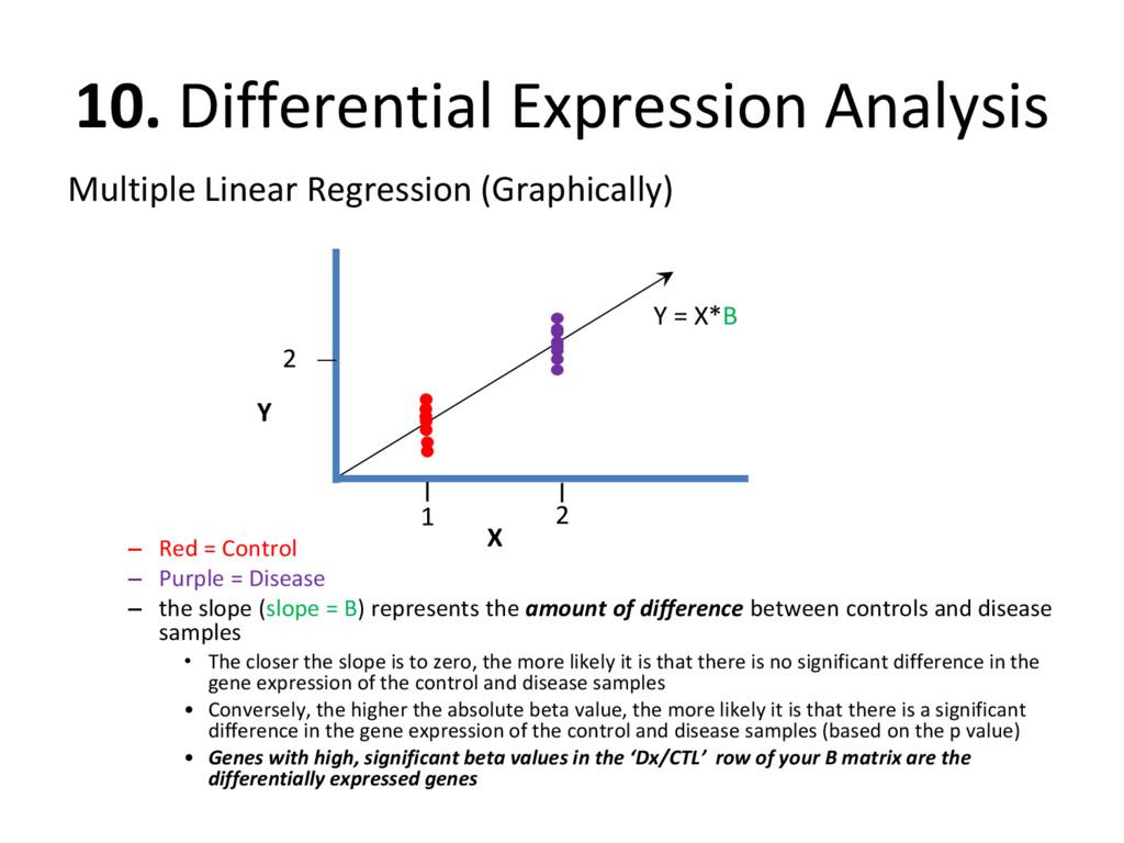
36. 10. Differential Expression Analysis Multiple Linear Regression (Graphically) – Red = Control – Purple = Disease – the slope (slope = B) represents the amount of difference between controls and disease samples • The closer the slope is to zero, the more likely it is that there is no significant difference in the gene expression of the control and disease samples • Conversely, the higher the absolute beta value, the more likely it is that there is a significant difference in the gene expression of the control and disease samples (based on the p value) • Genes with high, significant beta values in the ‘Dx/CTL’ row of your B matrix are the differentially expressed genes Y X 2 Y = X*B 1 2