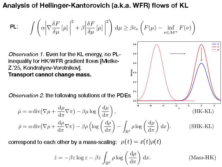
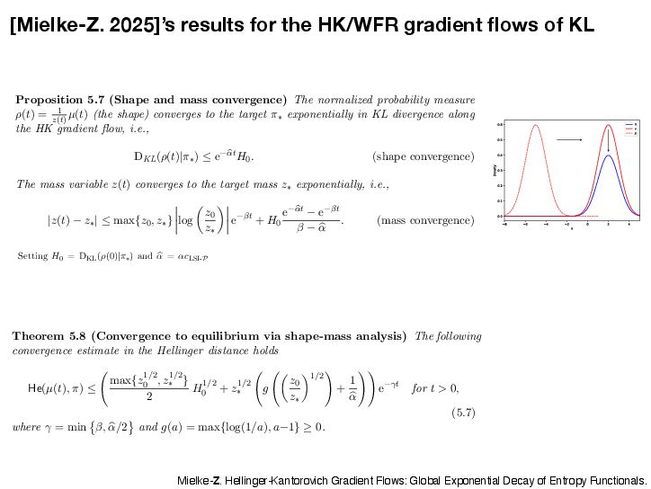
If DKL(ω(s)|ε→) → 0 for t → ↑, then h(t) → 0 and z(t) → z→. Setting H0 = D KL (ω(0)|ε→) and ϑ = ϑcLSI-P, we now deliver the convergence of the shape ω(t) to the target shape ε→ and the mass z(t) to the target mass z→. Proposition 5.7 (Shape and mass convergence) The normalized probability measure ω(t) = 1 z(t) µ(t) (the shape) converges to the target ε→ exponentially in KL divergence along the HK gradient flow, i.e., DKL(ω(t)|ε→) ↓ e↑εtH0. (shape convergence) The mass variable z(t) converges to the target mass z→ exponentially, i.e., |z(t) ↔ z→| ↓ max{z0, z→} log z0 z→ e↑ωt + H0 e↑εt ↔ e↑ωt ϖ ↔ ϑ . (mass convergence) Note that the convergence rate of the shape ω(t) to the limiting shape ε→ is dominated by the transport part alone, with an exponential decay rate ϑ = ϑCLSI . The total mass can only be changed by the growth through the Hellinger dissipation. Hence, the decay rate is simply ϖ, but it may be delayed by e↑εt if the shape converges only slowly. Combining the results of Proposition 5.6 and Proposition 5.7, we can now provide the global exponential decay analysis for the HK-KL gradient flow in the sense of the Hellinger distance. Theorem 5.8 (Convergence to equilibrium via shape-mass analysis) The following convergence estimate in the Hellinger distance holds He(µ(t), ε) ↓ max{z1/2 0 , z1/2 → } 2 H1/2 0 + z1/2 → g z0 z→ 1/2 + 1 ϑ e↑ϑt for t > 0, (5.7) where ϱ = min ϖ, ϑ/2 and g(a) = max{log(1/a), a↔1} ↗ 0. Setting H0 = D KL (ω(0)|ε→) and ϑ = ϑcLSI-P, we now deliver the convergence of the shape ω(t) to the target shape ε→ and the mass z(t) to the target mass z→. Proposition 5.7 (Shape and mass convergence) The normalized probability measure ω(t) = 1 z(t) µ(t) (the shape) converges to the target ε→ exponentially in KL divergence along the HK gradient flow, i.e., DKL(ω(t)|ε→) ↓ e↑εtH0. (shape convergence) The mass variable z(t) converges to the target mass z→ exponentially, i.e., |z(t) ↔ z→| ↓ max{z0, z→} log z0 z→ e↑ωt + H0 e↑εt ↔ e↑ωt ϖ ↔ ϑ . (mass convergence) Note that the convergence rate of the shape ω(t) to the limiting shape ε→ is dominated by the transport part alone, with an exponential decay rate ϑ = ϑCLSI . The total mass can only be changed by the growth through the Hellinger dissipation. Hence, the decay rate is simply ϖ, but it may be delayed by e↑εt if the shape converges only slowly. Combining the results of Proposition 5.6 and Proposition 5.7, we can now provide the global exponential decay analysis for the HK-KL gradient flow in the sense of the Hellinger distance. Theorem 5.8 (Convergence to equilibrium via shape-mass analysis) The following convergence estimate in the Hellinger distance holds He(µ(t), ε) ↓ max{z1/2 0 , z1/2 → } 2 H1/2 0 + z1/2 → g z0 z→ 1/2 + 1 ϑ e↑ϑt for t > 0, (5.7) where ϱ = min ϖ, ϑ/2 and g(a) = max{log(1/a), a↔1} ↗ 0. 35 [Mielke-Z. 2025]’s results for the HK/WFR gradient fl ows of KL HK Gradient Flows for Entropy Functionals Figure 7: See Proposition 5.2 for the details of the functional inequality a Wasserstein flow of positive measures. In this plot, the density rati constant. Hence, there is no “Otto-Wasserstein gradient” to drive the c ω towards ε. When initialized at µ, the Otto-Wasserstein flow drives towards ω. Proposition 5.3 (Generalized log-Sobolev inequality on M+) Suppose th mic Sobolev inequality (LSI) holds with a positive constant cLSI-P > 0 when res probability measures (i.e. µ and ε are probability measures). Then, the following holds for the Otto-Wasserstein gradient flow over the positive measures M+: → log dµ dε 2 dµ ↑ cLSI-P · D KL (µ|ε) ↓ (z log z ↓ z + 1) , ( where z := µ(!) is the total mass of the measure µ. Moreover, we have → log dµ dε 2 dµ ↑ cLSI-P · D KL (µ|z · ε) . The intuition here is that the Otto-Wasserstein gradient flow, viewed as a mass-p flow with total mass µ(!), satisfies the LSI type inequality. This is illustrated in Proof of Proposition 5.3. We have the logarithmic Sobolev inequality (LS probability measures ˜ µ := 1 z · µ where z := µ(!) is the mass of µ, d˜ µ dε → log d˜ µ dε 2 dε ↑ cLSI-P · D KL (˜ µ|ε). 31 HK Gradient Flows for Entropy Functionals In the following result, we can see two contributions to the convergence of µ(t) = z(t)ω(t) to ε = z→ε→, where z→ := ε(!) is the total mass of the target measure and ε→ is a probability measure, a.k.a. the shape. We now detail the results of the shape-mass analysis for the HK-KL gradient flow. We first provide the convergence of the mass variable z(t) to the target mass z→. Proposition 5.6 (Solution of the mass equation) The equation of mass (Mass-HK) admits the explicit solution z(t) = z→ z0 z→ e →ωt e↑h(t). (5.6) where h(t) = t 0 e↑ω(t↑s)DKL(ω(s)|ε→)ds is an auxiliary function. If DKL(ω(s)|ε→) → 0 for t → ↑, then h(t) → 0 and z(t) → z→. Setting H0 = D KL (ω(0)|ε→) and ϑ = ϑcLSI-P, we now deliver the convergence of the shape ω(t) to the target shape ε→ and the mass z(t) to the target mass z→. Proposition 5.7 (Shape and mass convergence) The normalized probability measure ω(t) = 1 z(t) µ(t) (the shape) converges to the target ε→ exponentially in KL divergence along the HK gradient flow, i.e., DKL(ω(t)|ε→) ↓ e↑εtH0. (shape convergence) The mass variable z(t) converges to the target mass z→ exponentially, i.e., |z(t) ↔ z→| ↓ max{z0, z→} log z0 z→ e↑ωt + H0 e↑εt ↔ e↑ωt ϖ ↔ ϑ . (mass convergence) Note that the convergence rate of the shape ω(t) to the limiting shape ε→ is dominated by the transport part alone, with an exponential decay rate ϑ = ϑCLSI . The total mass can only be changed by the growth through the Hellinger dissipation. Hence, the decay rate is simply ϖ, but it may be delayed by e↑εt if the shape converges only slowly. Combining the results of Proposition 5.6 and Proposition 5.7, we can now provide the Mielke-Z. Hellinger-Kantorovich Gradient Flows: Global Exponential Decay of Entropy Functionals.
![Theoretical analysis of Hellinger gradient flows [Z & Mielke ’24]](https://files.speakerdeck.com/presentations/e99b8fd444504c57b70d471565e60fde/slide_27.jpg)