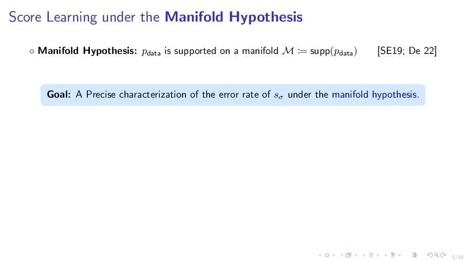
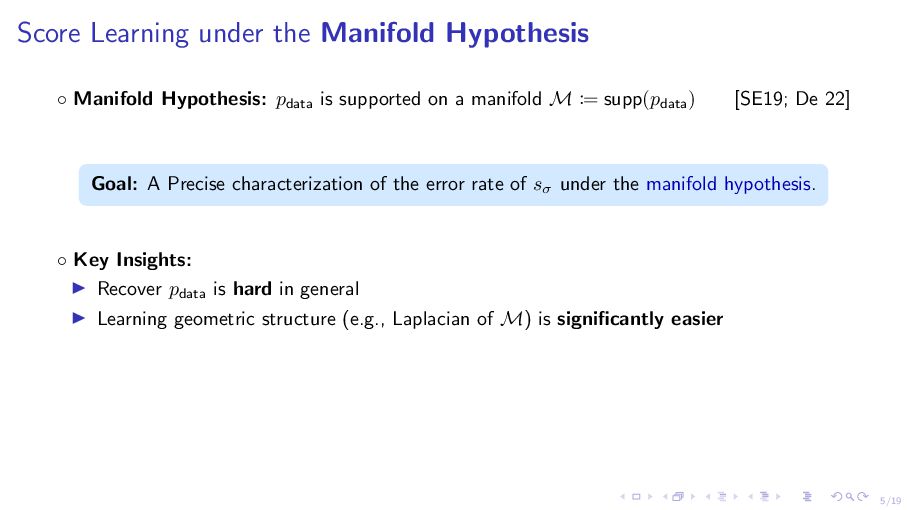
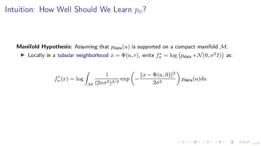
pdata is supported on a manifold M := supp(pdata) [SE19; De 22] Goal: A Precise characterization of the error rate of sσ under the manifold hypothesis.
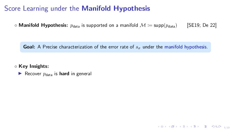
pdata is supported on a manifold M := supp(pdata) [SE19; De 22] Goal: A Precise characterization of the error rate of sσ under the manifold hypothesis. ◦ Key Insights: ▶ Recover pdata is hard in general
pdata is supported on a manifold M := supp(pdata) [SE19; De 22] Goal: A Precise characterization of the error rate of sσ under the manifold hypothesis. ◦ Key Insights: ▶ Recover pdata is hard in general ▶ Learning geometric structure (e.g., Laplacian of M) is significantly easier
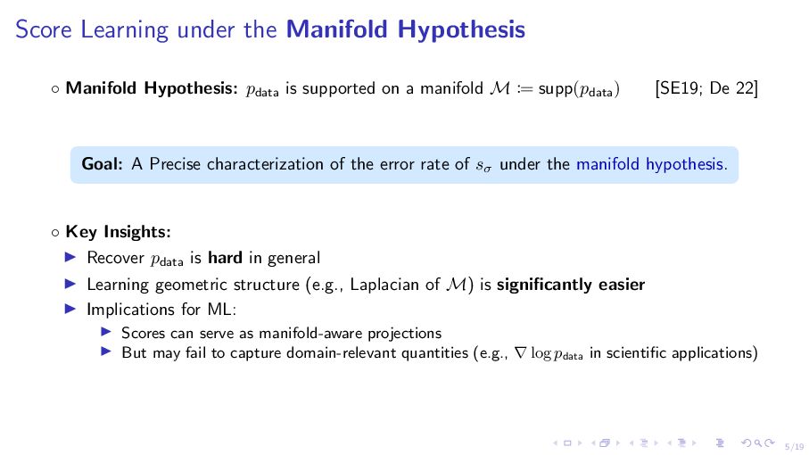
pdata is supported on a manifold M := supp(pdata) [SE19; De 22] Goal: A Precise characterization of the error rate of sσ under the manifold hypothesis. ◦ Key Insights: ▶ Recover pdata is hard in general ▶ Learning geometric structure (e.g., Laplacian of M) is significantly easier ▶ Implications for ML: ▶ Scores can serve as manifold-aware projections ▶ But may fail to capture domain-relevant quantities (e.g., ∇ log pdata in scientific applications)
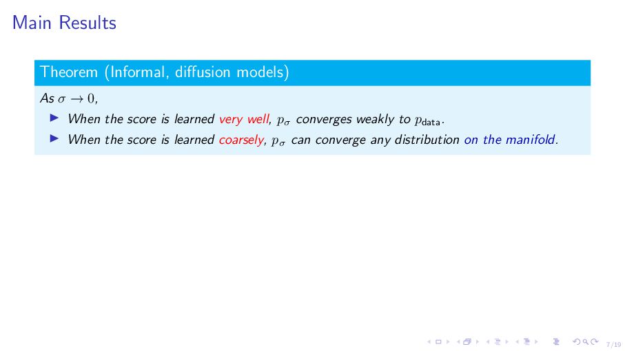
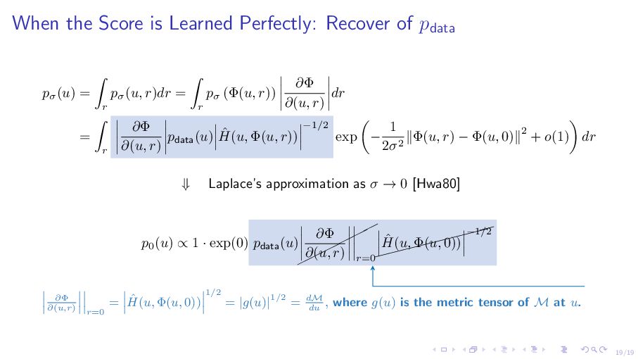
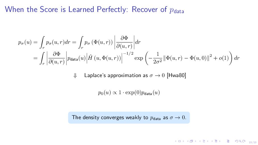
0, ▶ When the score is learned very well, pσ converges weakly to pdata . ▶ When the score is learned coarsely, pσ can converge any distribution on the manifold.
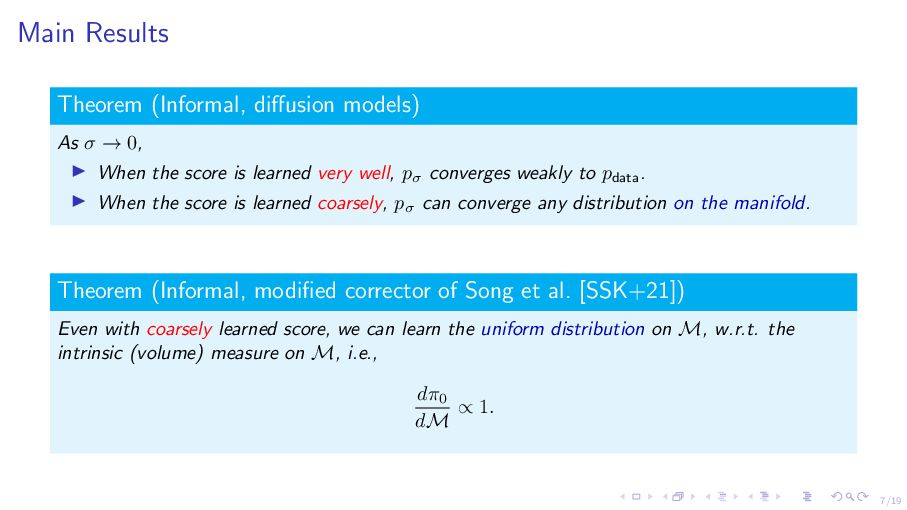
0, ▶ When the score is learned very well, pσ converges weakly to pdata . ▶ When the score is learned coarsely, pσ can converge any distribution on the manifold. Theorem (Informal, modified corrector of Song et al. [SSK+21]) Even with coarsely learned score, we can learn the uniform distribution on M, w.r.t. the intrinsic (volume) measure on M, i.e., dπ0 dM ∝ 1.
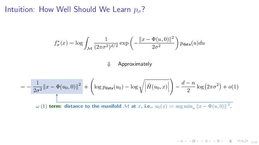
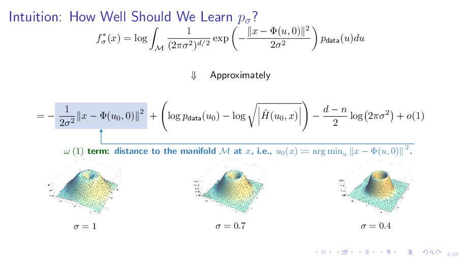
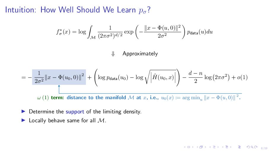
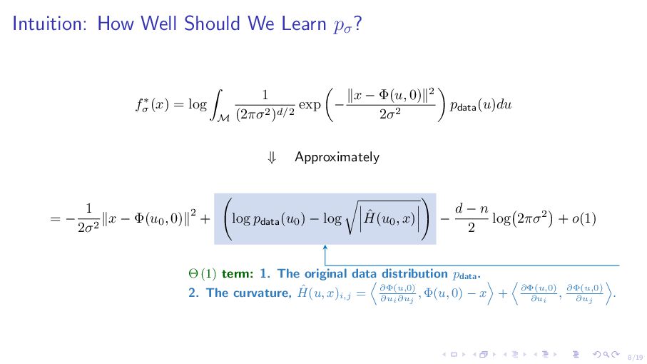
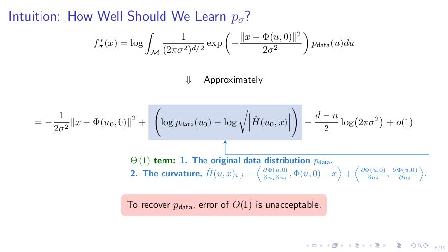
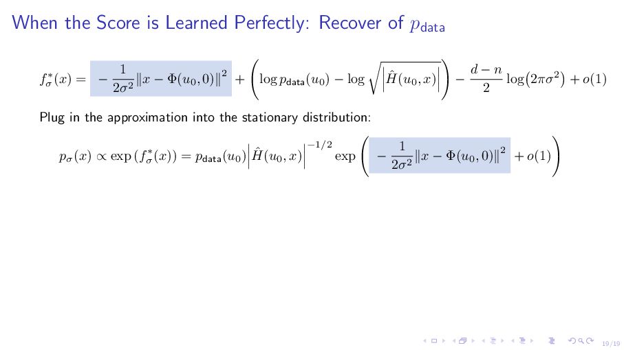
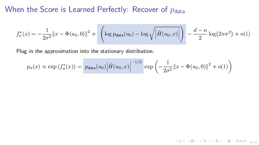
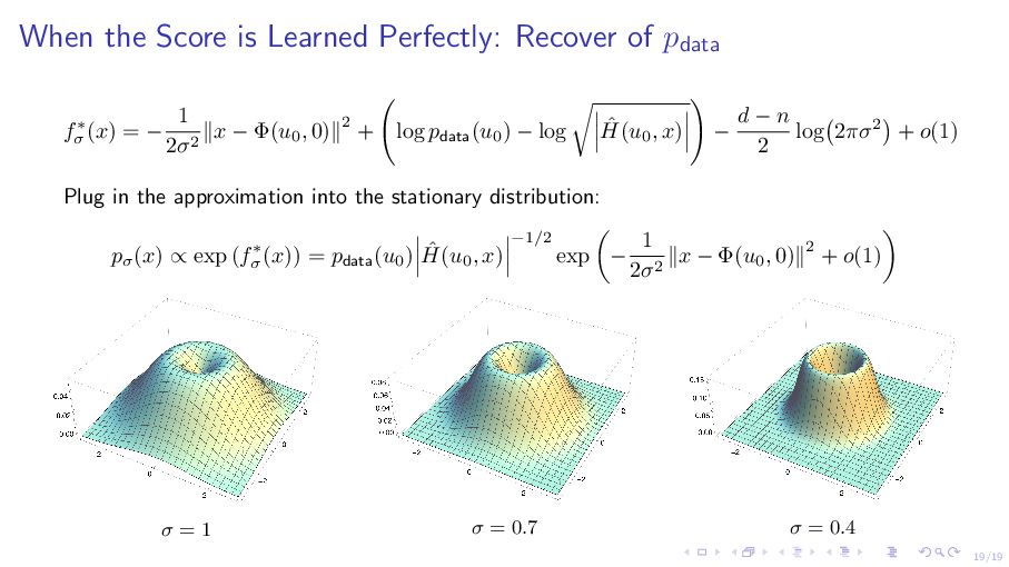
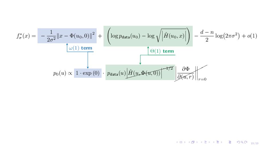
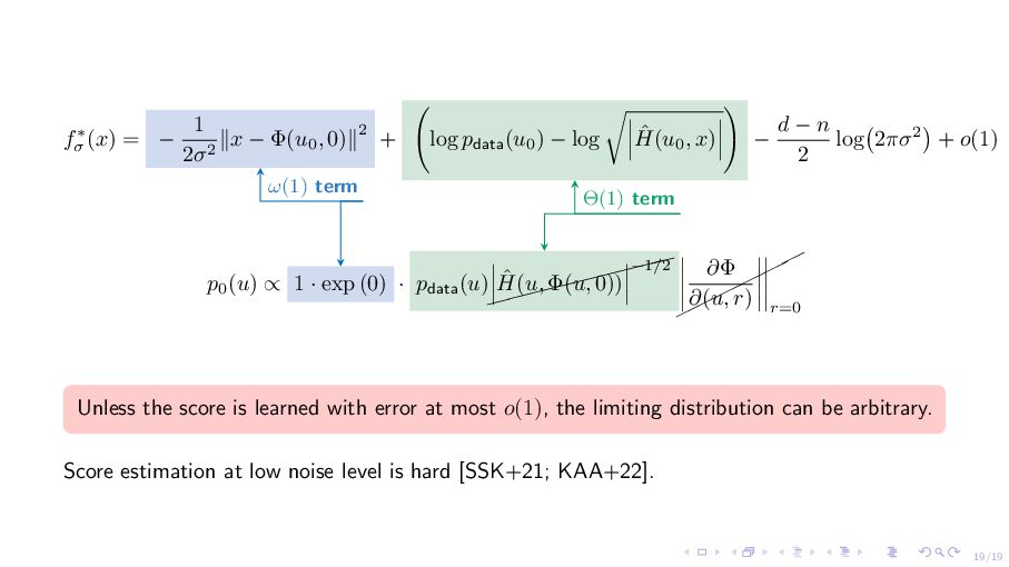
σ (x) = log M 1 (2πσ2)d/2 exp − ∥x − Φ(u, 0)∥2 2σ2 pdata(u)du ⇓ Approximately = − 1 2σ2 ∥x − Φ(u0 , 0)∥2 + log pdata(u0 ) − log ˆ H(u0 , x) − d − n 2 log 2πσ2 + o(1) ω (1) term: distance to the manifold M at x, i.e., u0 (x) := arg minu ∥x − Φ(u, 0)∥ 2. ▶ Determine the support of the limiting density. ▶ Locally behave same for all M.
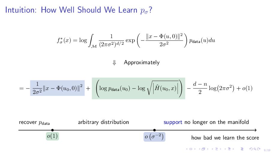
σ (x) = log M 1 (2πσ2)d/2 exp − ∥x − Φ(u, 0)∥2 2σ2 pdata(u)du ⇓ Approximately = − 1 2σ2 ∥x − Φ(u0 , 0)∥2 + log pdata(u0 ) − log ˆ H(u0 , x) − d − n 2 log 2πσ2 + o(1) how bad we learn the score o(1) o σ−2 recover pdata arbitrary distribution support no longer on the manifold
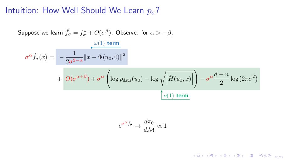
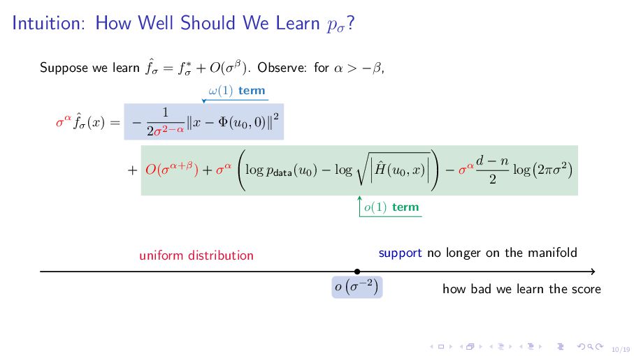
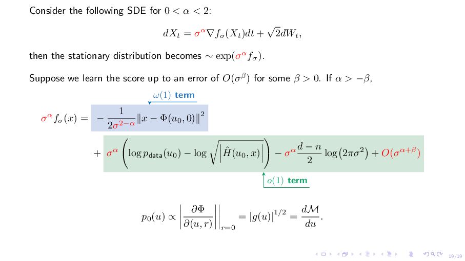
we learn ˆ fσ = f∗ σ + O(σβ). Observe: for α > −β, σα ˆ fσ (x) = − 1 2σ2−α ∥x − Φ(u0 , 0)∥2 + O(σα+β) + σα log pdata(u0 ) − log ˆ H(u0 , x) − σα d − n 2 log 2πσ2 ω(1) term o(1) term how bad we learn the score o σ−2 uniform distribution support no longer on the manifold
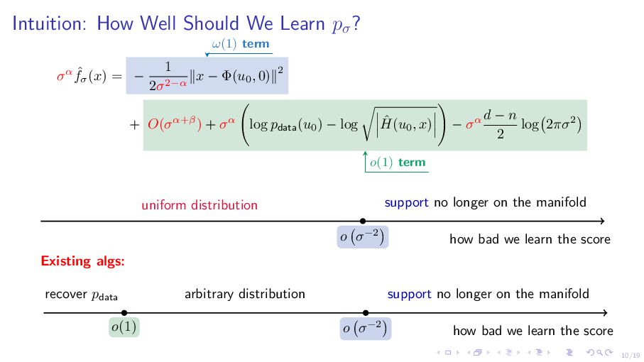
ˆ fσ (x) = − 1 2σ2−α ∥x − Φ(u0 , 0)∥2 + O(σα+β) + σα log pdata(u0 ) − log ˆ H(u0 , x) − σα d − n 2 log 2πσ2 ω(1) term o(1) term how bad we learn the score o σ−2 uniform distribution support no longer on the manifold Existing algs: how bad we learn the score o(1) o σ−2 recover pdata arbitrary distribution support no longer on the manifold
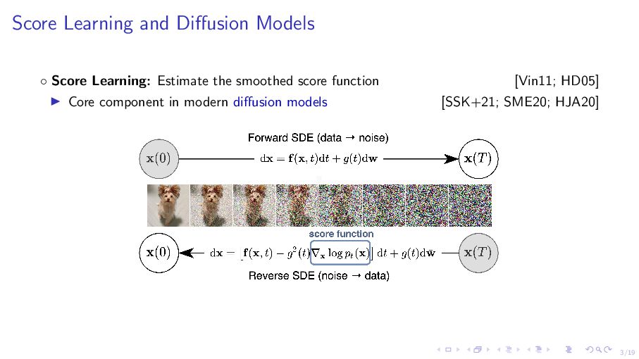
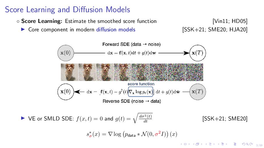
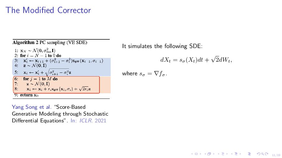
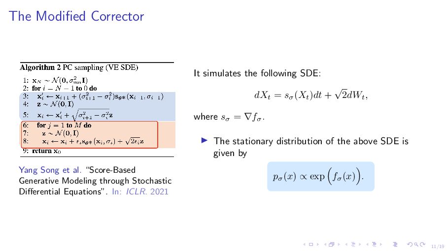
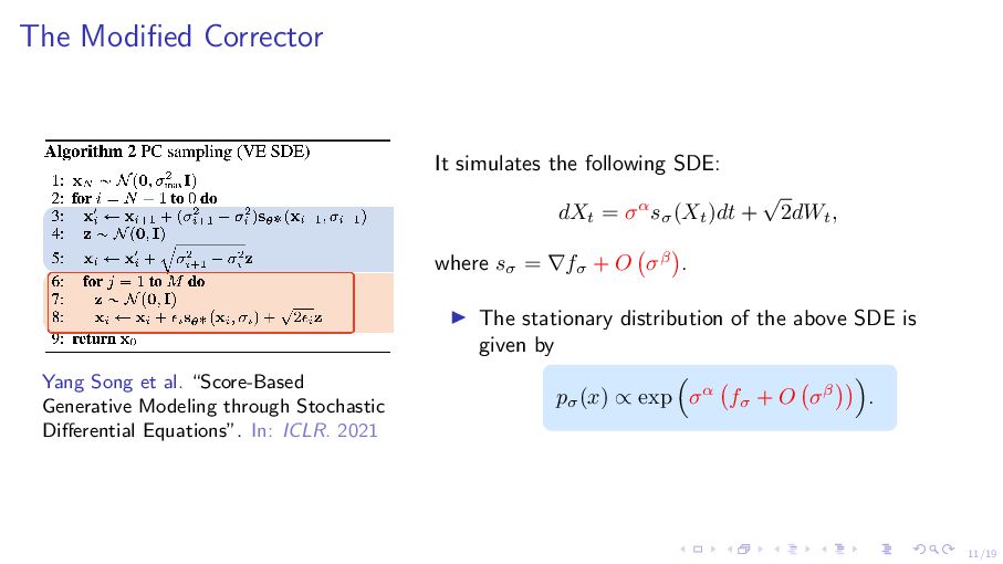
Modeling through Stochastic Differential Equations”. In: ICLR. 2021 It simulates the following SDE: dXt = sσ (Xt )dt + √ 2dWt , where sσ = ∇fσ . ▶ The stationary distribution of the above SDE is given by pσ (x) ∝ exp fσ (x) .
Modeling through Stochastic Differential Equations”. In: ICLR. 2021 It simulates the following SDE: dXt = σαsσ (Xt )dt + √ 2dWt , where sσ = ∇fσ + O σβ . ▶ The stationary distribution of the above SDE is given by pσ (x) ∝ exp σα fσ + O σβ .
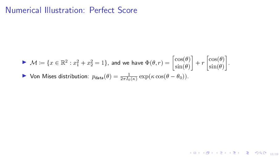
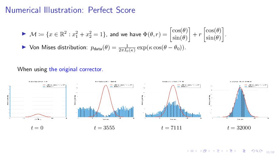
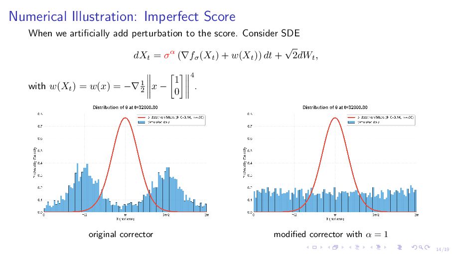
R2 : x2 1 + x2 2 = 1}, and we have Φ(θ, r) = cos(θ) sin(θ) + r cos(θ) sin(θ) . ▶ Von Mises distribution: pdata(θ) = 1 2πI0(κ) exp(κ cos(θ − θ0 )). When using the original corrector. t = 0 t = 3555 t = 7111 t = 32000
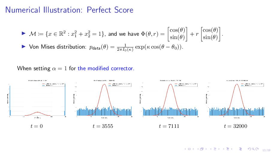
R2 : x2 1 + x2 2 = 1}, and we have Φ(θ, r) = cos(θ) sin(θ) + r cos(θ) sin(θ) . ▶ Von Mises distribution: pdata(θ) = 1 2πI0(κ) exp(κ cos(θ − θ0 )). When setting α = 1 for the modified corrector. t = 0 t = 3555 t = 7111 t = 32000
interesting properties. ▶ Leading term being the distance to the manifold. ▶ The original distribution is in higher order terms (making it hard to recover). ▶ Learning the manifold is significantly easier than learning the data distribution.
Zugner, Marco Federici, Cecilia Clementi, Frank No´ e, Robert Pinsler, and Rianne van den Berg. “Two for one: Diffusion models and force fields for coarse-grained molecular dynamics”. In: Journal of Chemical Theory and Computation 19.18 (2023), pp. 6151–6159. [De 22] Valentin De Bortoli. “Convergence of denoising diffusion models under the manifold hypothesis”. In: arXiv preprint arXiv:2208.05314 (2022). [HD05] Aapo Hyv¨ arinen and Peter Dayan. “Estimation of non-normalized statistical models by score matching.”. In: Journal of Machine Learning Research 6.4 (2005). [HJA20] Jonathan Ho, Ajay Jain, and Pieter Abbeel. “Denoising diffusion probabilistic models”. In: Advances in neural information processing systems 33 (2020), pp. 6840–6851. [Hwa80] Chii-Ruey Hwang. “Laplace’s method revisited: weak convergence of probability measures”. In: The Annals of Probability (1980), pp. 1177–1182. [KAA+22] Tero Karras, Miika Aittala, Timo Aila, and Samuli Laine. “Elucidating the design space of diffusion-based generative models”. In: Advances in neural information processing systems 35 (2022), pp. 26565–26577.
Psenka, Tobias Kreiman, Michal Pavelka, and Aditi S Krishnapriyan. “Action-Minimization Meets Generative Modeling: Efficient Transition Path Sampling with the Onsager-Machlup Functional”. In: arXiv preprint arXiv:2504.18506 (2025). [SBD+24] Jan Pawel Stanczuk, Georgios Batzolis, Teo Deveney, and Carola-Bibiane Sch¨ onlieb. “Diffusion models encode the intrinsic dimension of data manifolds”. In: Forty-first International Conference on Machine Learning. 2024. [SE19] Yang Song and Stefano Ermon. “Generative modeling by estimating gradients of the data distribution”. In: Advances in neural information processing systems 32 (2019). [SME20] Jiaming Song, Chenlin Meng, and Stefano Ermon. “Denoising diffusion implicit models”. In: arXiv preprint arXiv:2010.02502 (2020). [SSK+21] Yang Song, Jascha Sohl-Dickstein, Diederik P Kingma, Abhishek Kumar, Stefano Ermon, and Ben Poole. “Score-Based Generative Modeling through Stochastic Differential Equations”. In: ICLR. 2021. [Vin11] Pascal Vincent. “A connection between score matching and denoising autoencoders”. In: Neural computation 23.7 (2011), pp. 1661–1674.
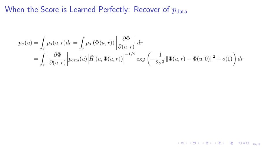
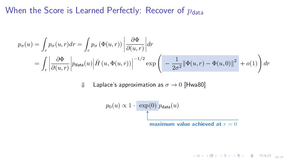
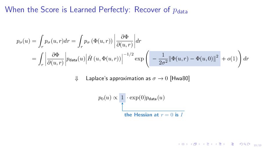
Φ(u0 , 0)∥2 + log pdata(u0 ) − log ˆ H(u0 , x) − d − n 2 log 2πσ2 + o(1) p0 (u) ∝ 1 · exp (0) · pdata(u) $$$$$$$$ $ ˆ H(u, Φ(u, 0)) −1/2 ¨¨¨ ¨¨ ¨ ∂Φ ∂(u, r) r=0 ω(1) term Θ(1) term Unless the score is learned with error at most o(1), the limiting distribution can be arbitrary. Score estimation at low noise level is hard [SSK+21; KAA+22].
![18/19 [AGH+23] Marloes Arts, Victor Garcia Satorras, Chin-Wei Huang, Daniel](https://files.speakerdeck.com/presentations/22a26a5cbb94422a8ba57b4df216f6a0/slide_35.jpg)
![19/19 [Rˇ SP+25] Sanjeev Raja, Martin ˇ S´ ıpka, Michael](https://files.speakerdeck.com/presentations/22a26a5cbb94422a8ba57b4df216f6a0/slide_36.jpg)