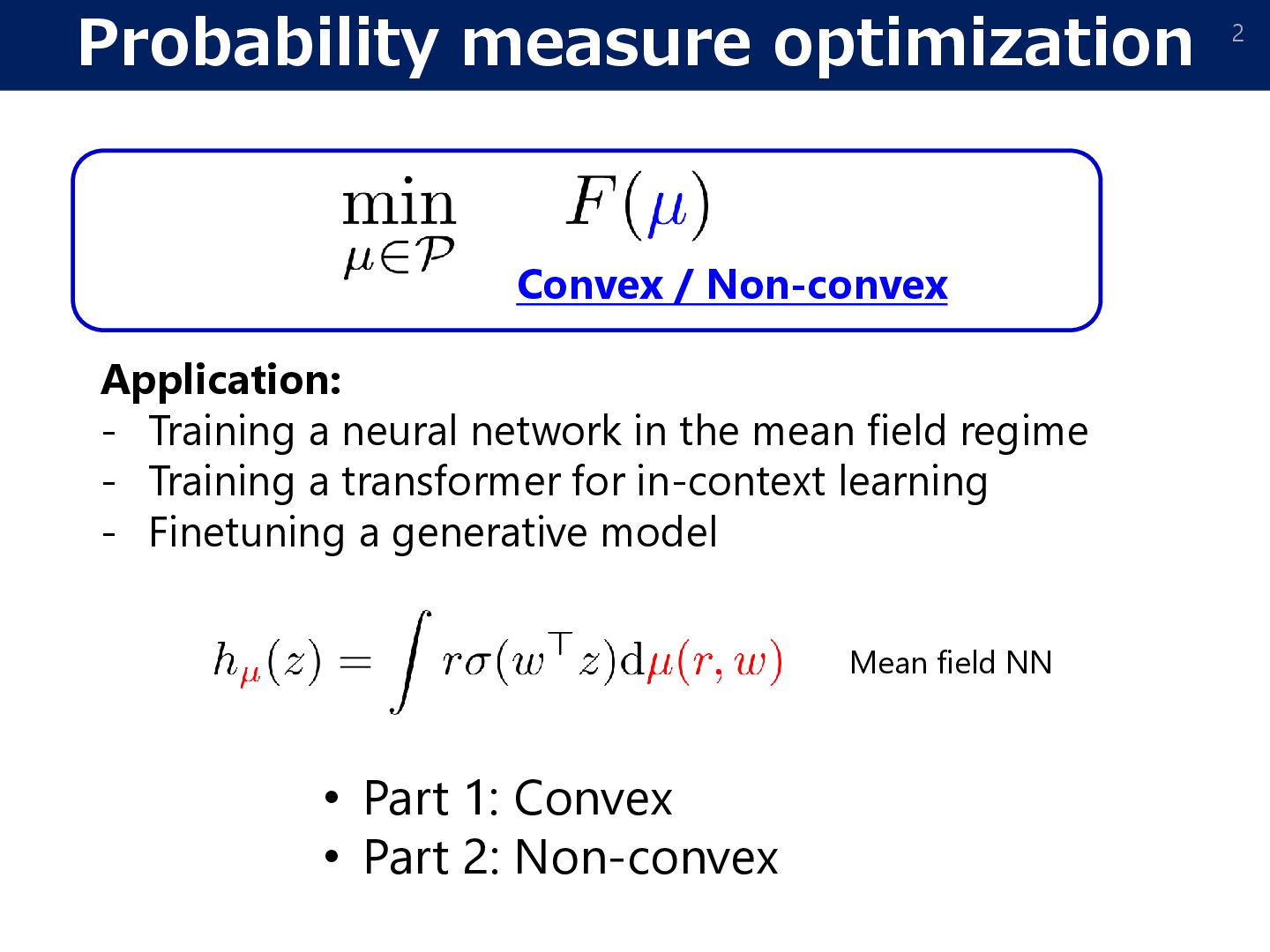
a neural network in the mean field regime - Training a transformer for in-context learning - Finetuning a generative model Mean field NN • Part 1: Convex • Part 2: Non-convex
Sakaguchi, Suzuki: Propagation of Chaos for Mean-Field Langevin Dynamics and its Application to Model Ensemble. ICML2025. • [Optimization of a probability measure on a strict saddle objecive] - Kim, Suzuki: Transformers Learn Nonlinear Features In Context: Nonconvex Mean-field Dynamics on the Attention Landscape. ICML2024, oral. - Yamamto, Kim, Suzuki: Hessian-guided Perturbed Wasserstein Gradient Flows for Escaping Saddle Points. 2025. Part 2: Non-convex (strict-saddle objective) 1. Gaussian process perturbation: A polynomial time method to avoid a saddle point by a “random perturbation” of a probability measure. 2. In-context learning: The objective to train a two-layer transformer is strict-saddle. Mean-field Langevin dynamics (𝐹 𝜇 + 𝜆Ent(𝜇)) • Optimization of probability measures by WG-flow • Particle approximation • Defective log-Sobolev inequality Part 1: Convex (propagation of chaos)
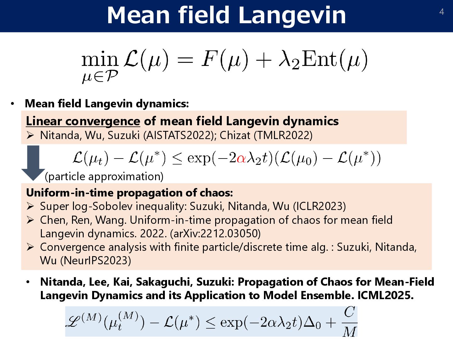
dynamics ➢ Nitanda, Wu, Suzuki (AISTATS2022); Chizat (TMLR2022) Uniform-in-time propagation of chaos: ➢ Super log-Sobolev inequality: Suzuki, Nitanda, Wu (ICLR2023) ➢ Chen, Ren, Wang. Uniform-in-time propagation of chaos for mean field Langevin dynamics. 2022. (arXiv:2212.03050) ➢ Convergence analysis with finite particle/discrete time alg. : Suzuki, Nitanda, Wu (NeurIPS2023) (particle approximation) • Mean field Langevin dynamics: • Nitanda, Lee, Kai, Sakaguchi, Suzuki: Propagation of Chaos for Mean-Field Langevin Dynamics and its Application to Model Ensemble. ICML2025.
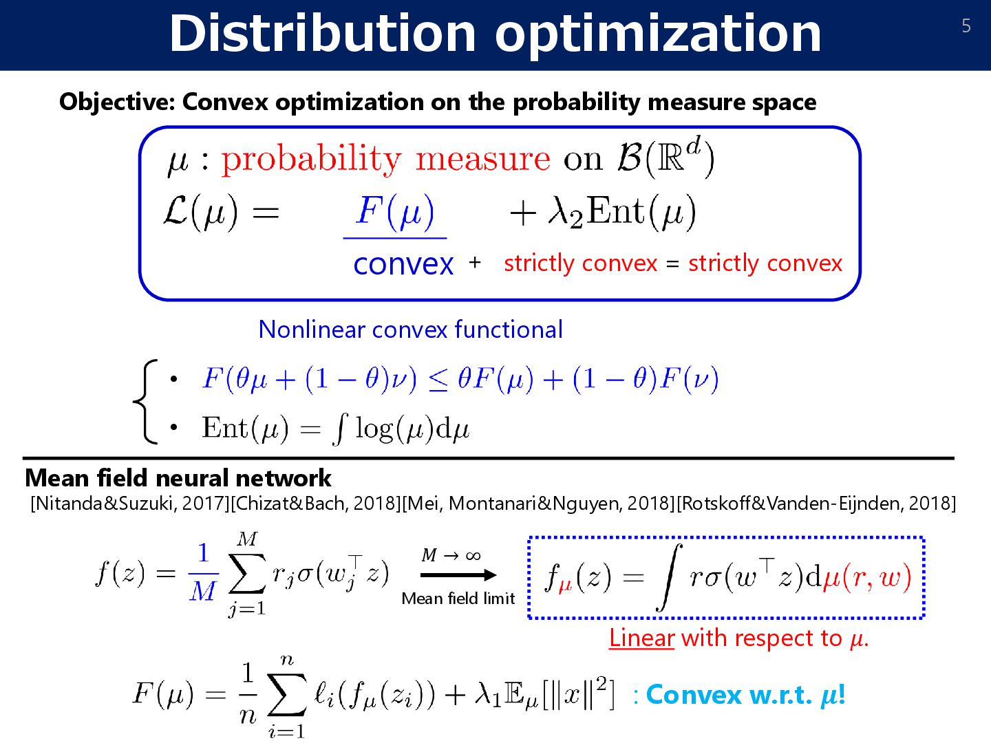
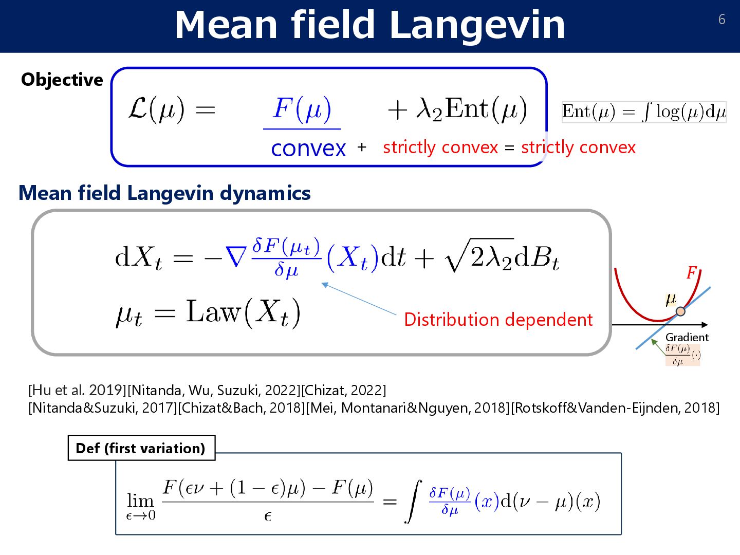
the probability measure space convex strictly convex = strictly convex + • • [Nitanda&Suzuki, 2017][Chizat&Bach, 2018][Mei, Montanari&Nguyen, 2018][Rotskoff&Vanden-Eijnden, 2018] 𝑀 → ∞ Linear with respect to 𝜇. Mean field neural network : Convex w.r.t. 𝝁! Mean field limit
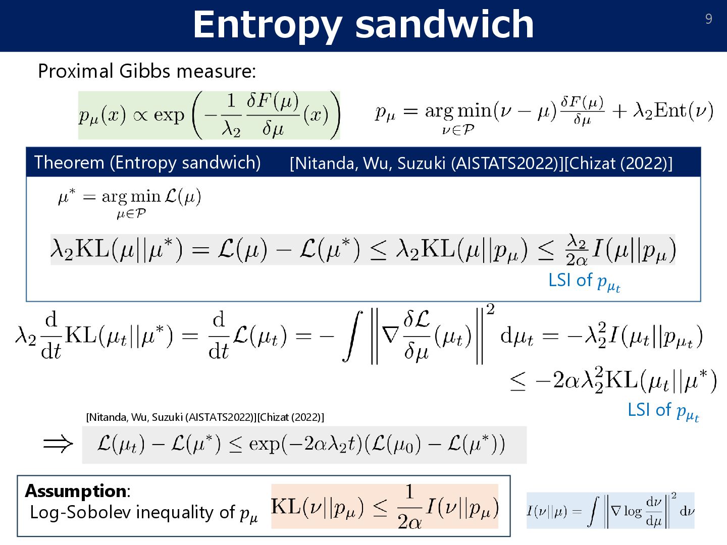
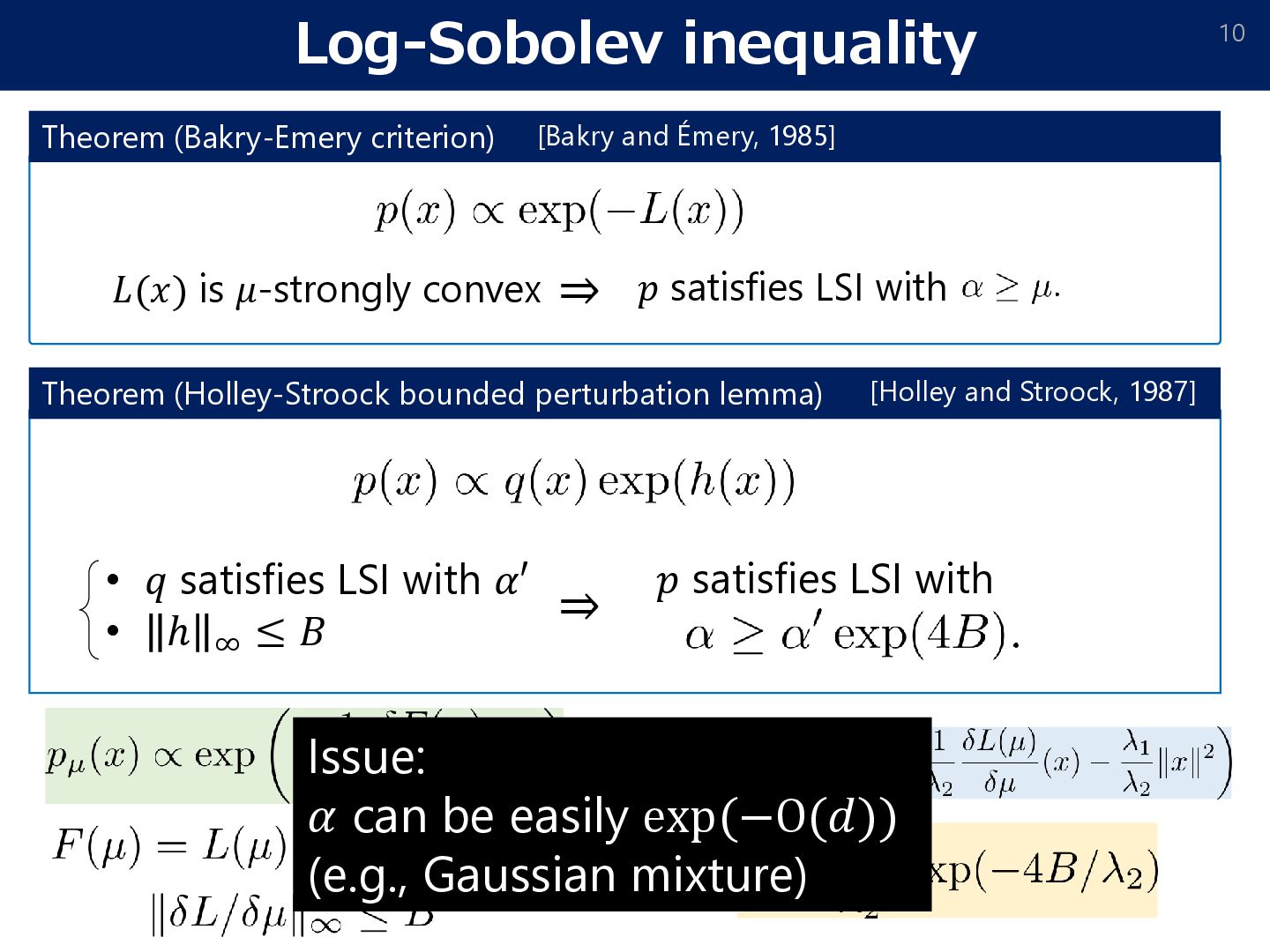
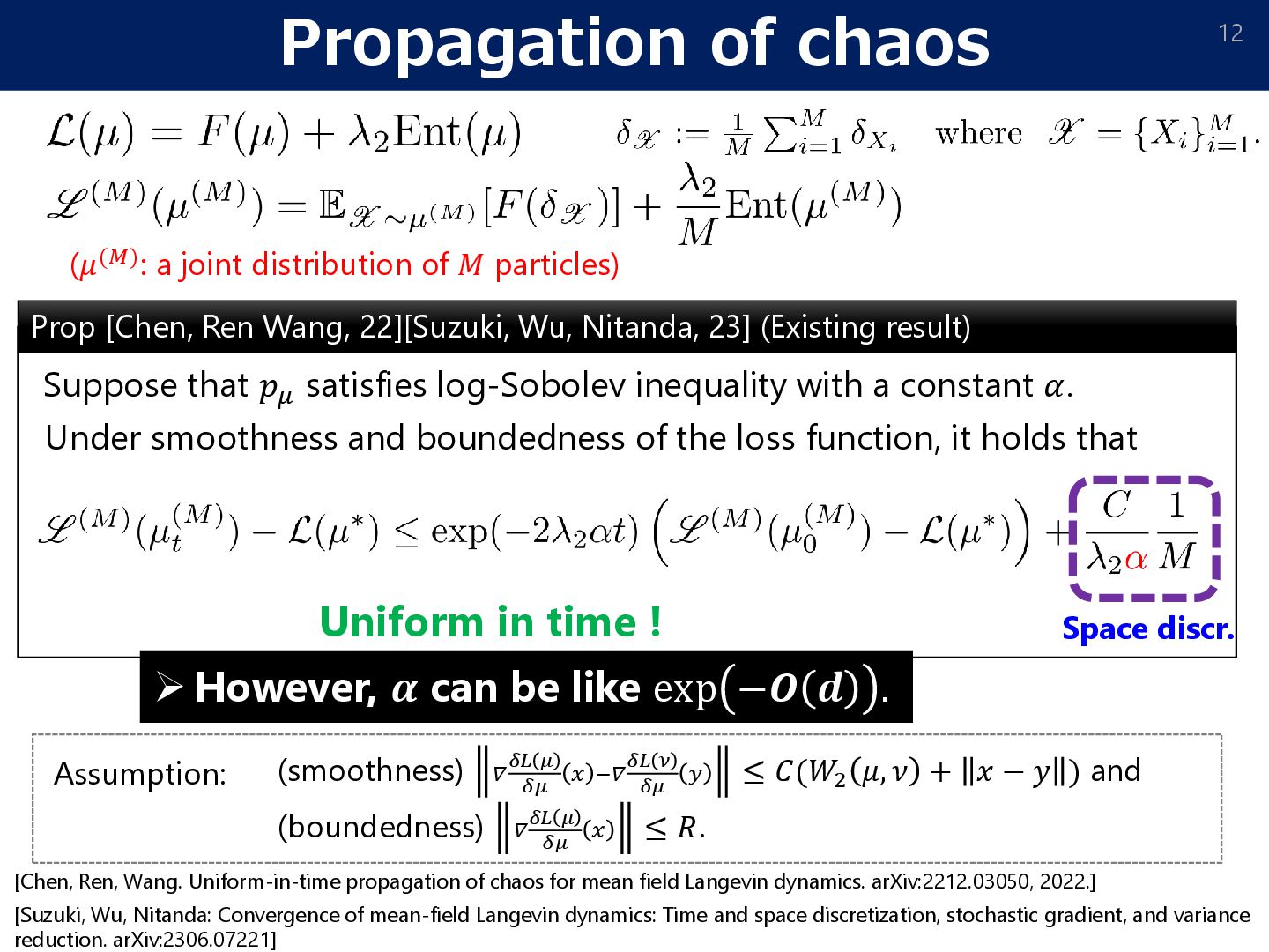
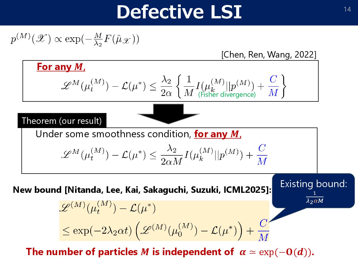
of the loss function, it holds that Suppose that 𝑝𝜇 satisfies log-Sobolev inequality with a constant 𝛼. Prop [Chen, Ren Wang, 22][Suzuki, Wu, Nitanda, 23] (Existing result) (smoothness) 𝛻𝛿𝐿 𝜇 𝛿𝜇 𝑥 −𝛻𝛿𝐿 𝜈 𝛿𝜇 𝑦 ≤ 𝐶(𝑊2 𝜇, 𝜈 + 𝑥 − 𝑦 ) and (boundedness) 𝛻𝛿𝐿 𝜇 𝛿𝜇 𝑥 ≤ 𝑅. Assumption: [Suzuki, Wu, Nitanda: Convergence of mean-field Langevin dynamics: Time and space discretization, stochastic gradient, and variance reduction. arXiv:2306.07221] [Chen, Ren, Wang. Uniform-in-time propagation of chaos for mean field Langevin dynamics. arXiv:2212.03050, 2022.] ➢However, 𝜶 can be like exp −𝑶 𝒅 . (𝜇(𝑀): a joint distribution of 𝑀 particles) Uniform in time !
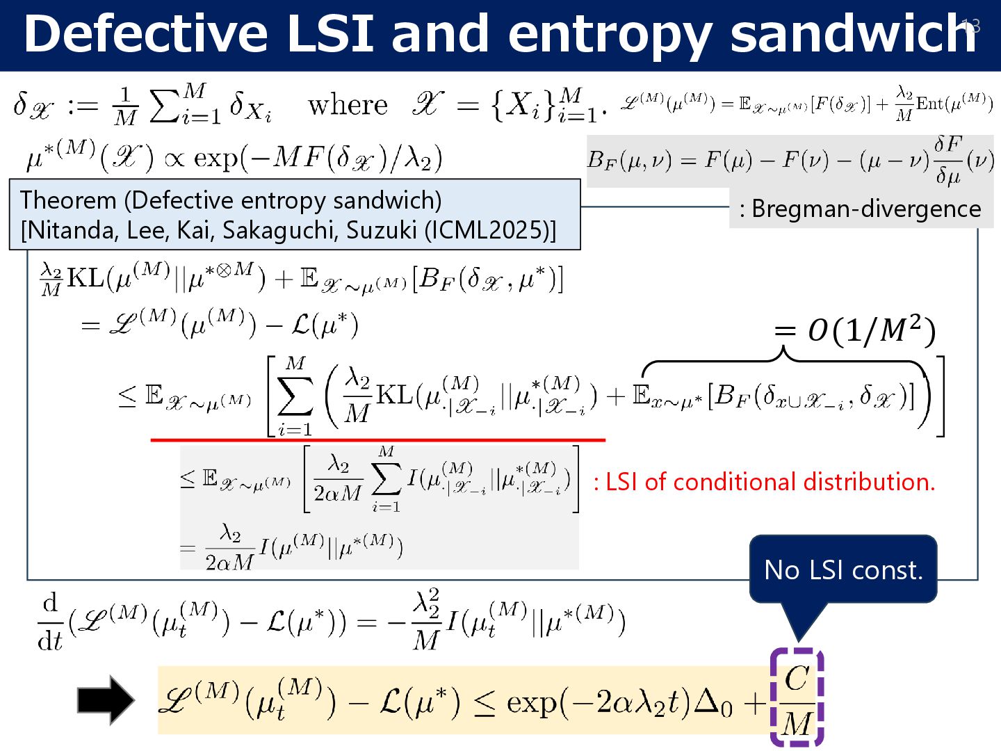
smoothness condition, for any 𝑴, Theorem (our result) New bound [Nitanda, Lee, Kai, Sakaguchi, Suzuki, ICML2025]: The number of particles 𝑴 is independent of 𝜶 ≃ exp(−𝚶(𝒅)). Existing bound: 1 𝜆2𝛼𝑀 [Chen, Ren, Wang, 2022]
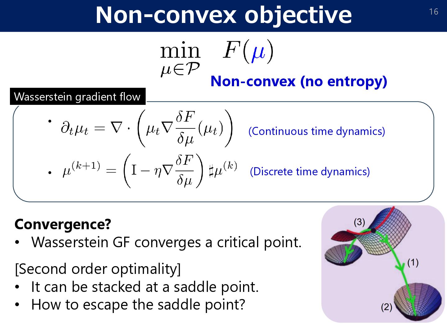
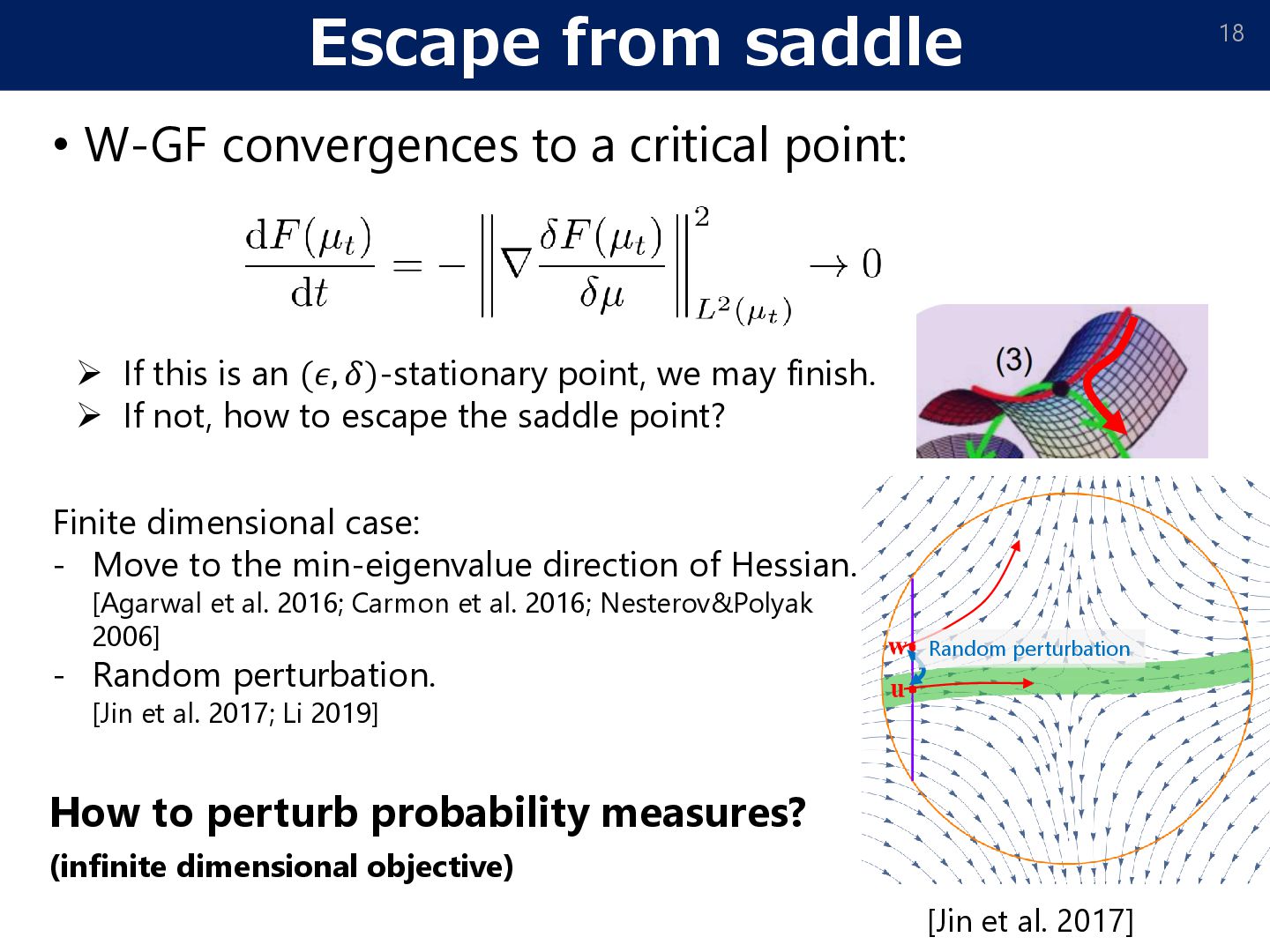
• Wasserstein GF converges a critical point. [Second order optimality] • It can be stacked at a saddle point. • How to escape the saddle point? Wasserstein gradient flow • • Non-convex (no entropy)
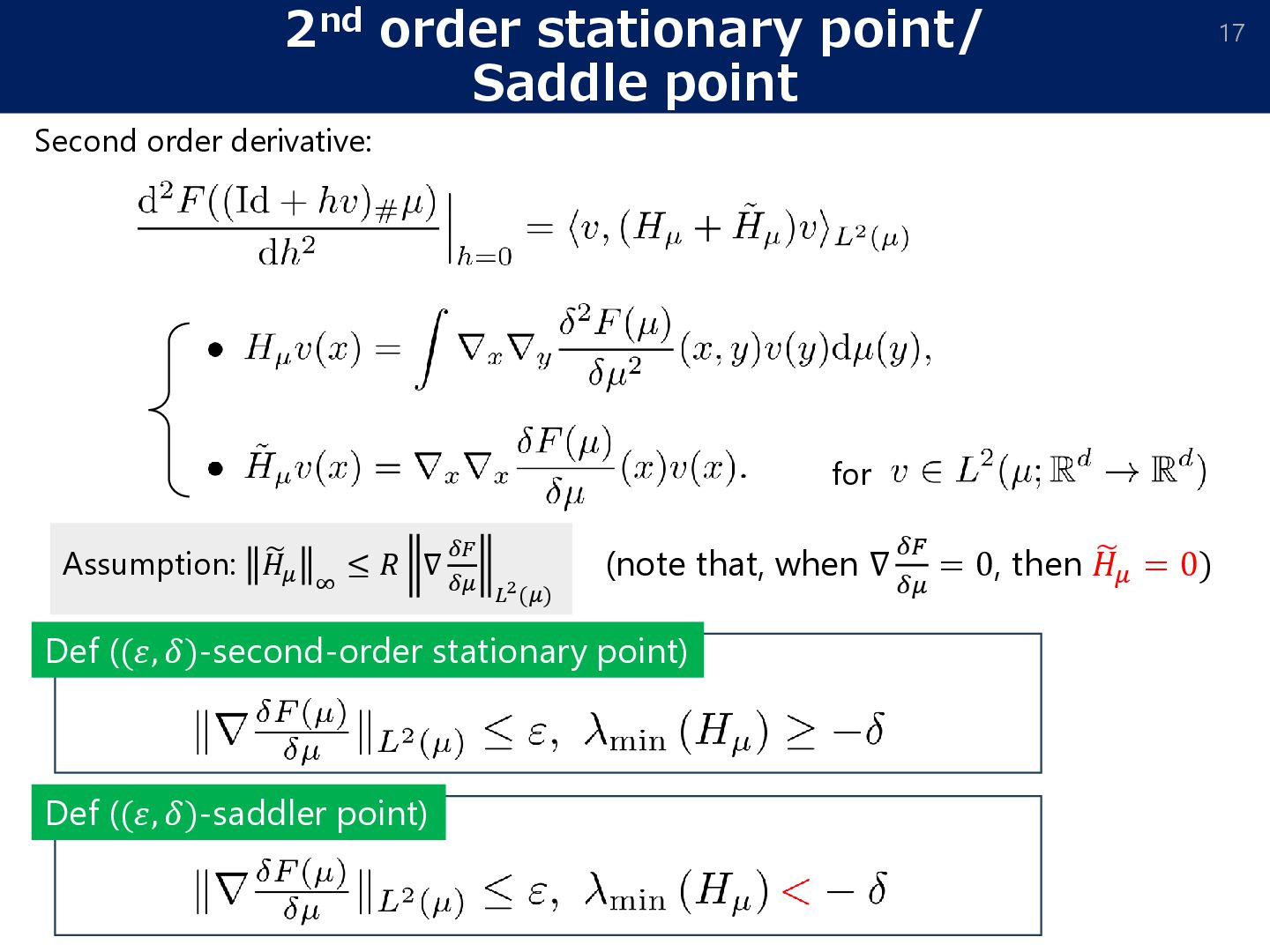
18 ➢ If this is an (𝜖, 𝛿)-stationary point, we may finish. ➢ If not, how to escape the saddle point? Finite dimensional case: - Move to the min-eigenvalue direction of Hessian. [Agarwal et al. 2016; Carmon et al. 2016; Nesterov&Polyak 2006] - Random perturbation. [Jin et al. 2017; Li 2019] [Jin et al. 2017] How to perturb probability measures? (infinite dimensional objective) Random perturbation
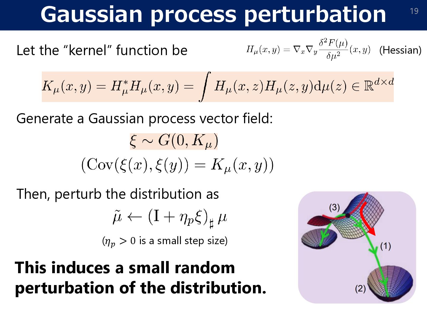
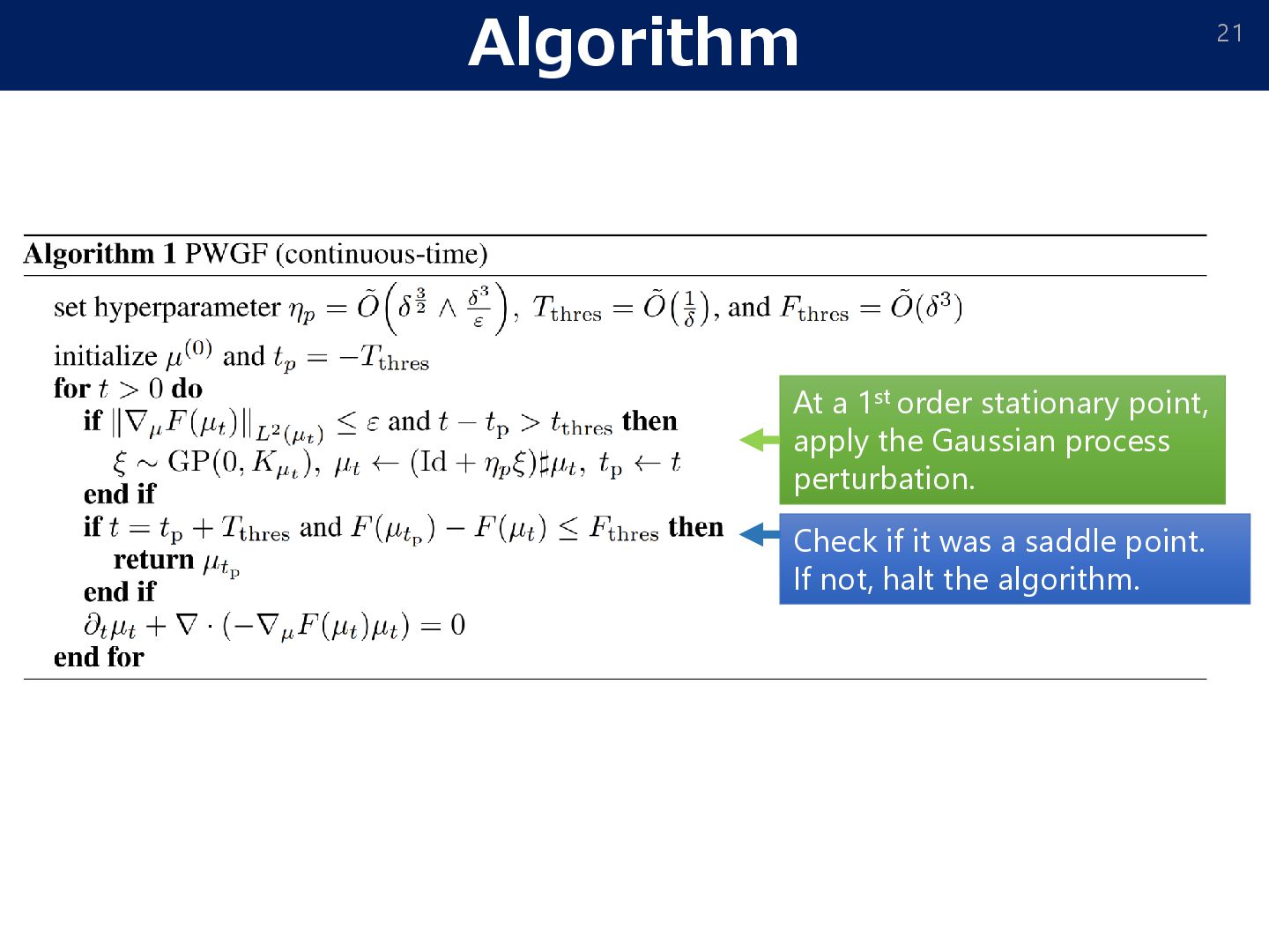
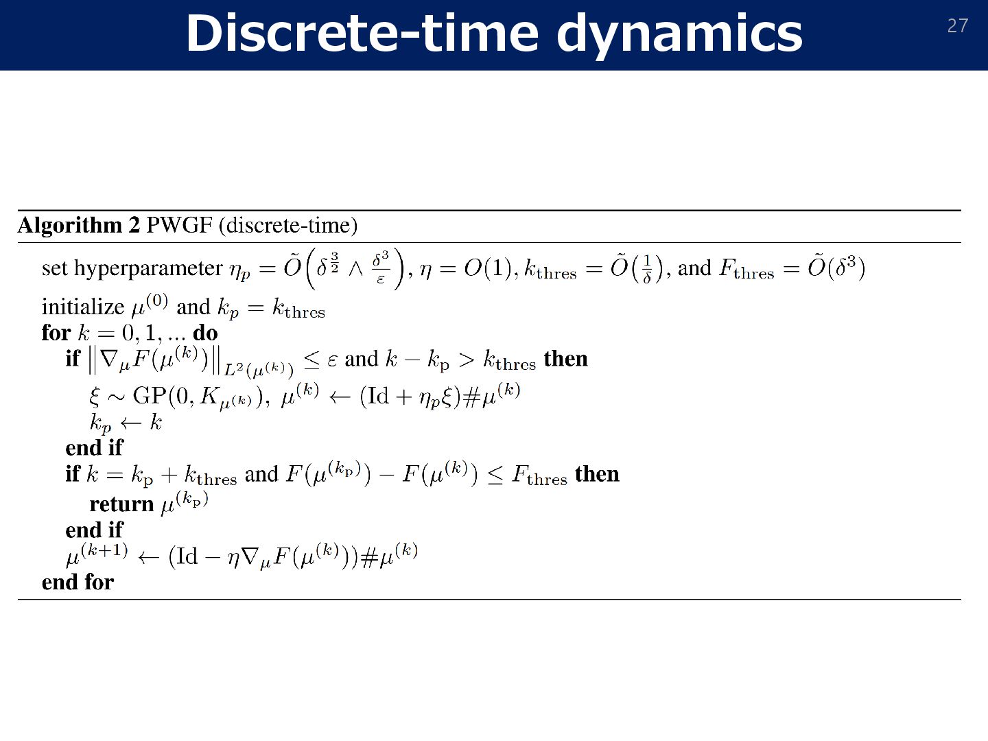
a Gaussian process vector field: Then, perturb the distribution as This induces a small random perturbation of the distribution. (𝜂𝑝 > 0 is a small step size) (Hessian)
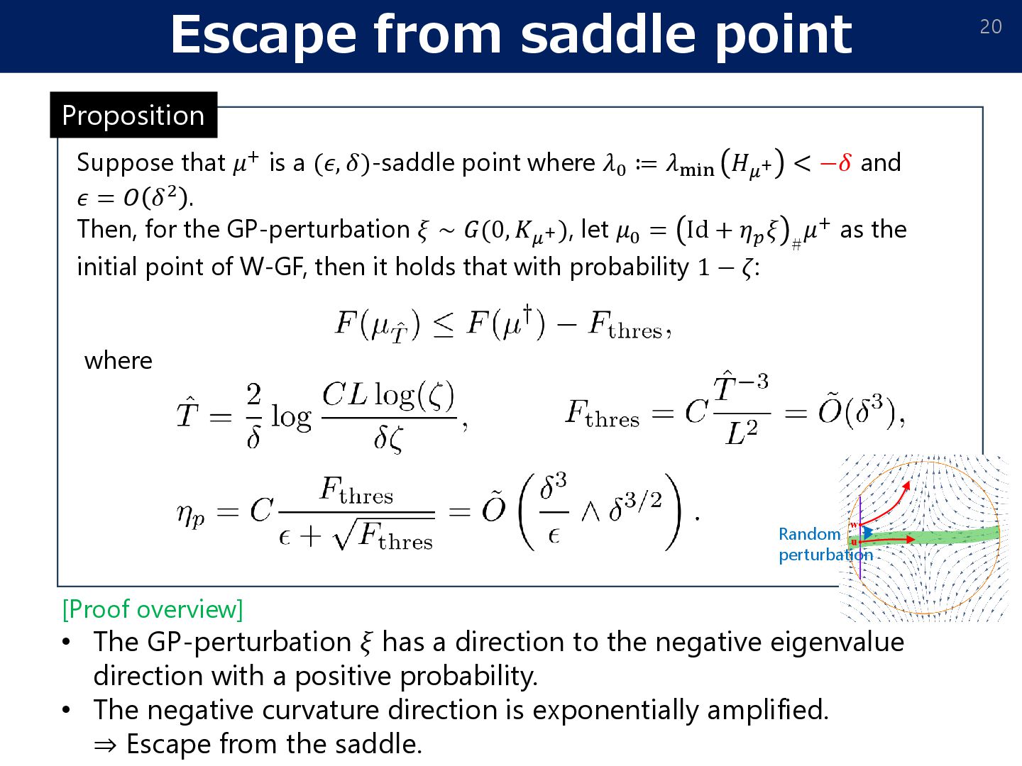
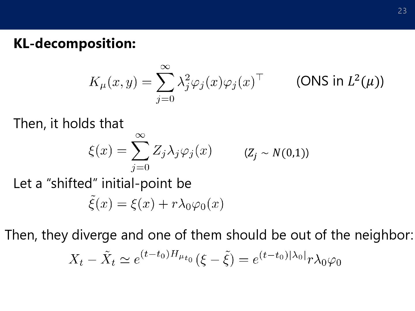
a (𝜖, 𝛿)-saddle point where 𝜆0 ≔ 𝜆min 𝐻𝜇+ < −𝛿 and 𝜖 = 𝑂 𝛿2 . Then, for the GP-perturbation 𝜉 ∼ 𝐺(0, 𝐾𝜇+), let 𝜇0 = Id + 𝜂𝑝 𝜉 # 𝜇+ as the initial point of W-GF, then it holds that with probability 1 − 𝜁: where [Proof overview] • The GP-perturbation 𝜉 has a direction to the negative eigenvalue direction with a positive probability. • The negative curvature direction is exponentially amplified. ⇒ Escape from the saddle. Random perturbation
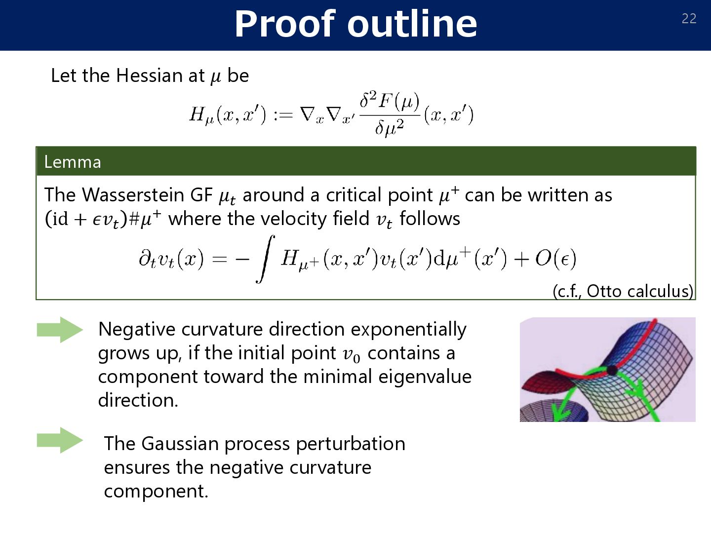
The Wasserstein GF 𝜇𝑡 around a critical point 𝜇+ can be written as id + 𝜖𝑣𝑡 #𝜇+ where the velocity field 𝑣𝑡 follows Negative curvature direction exponentially grows up, if the initial point 𝑣0 contains a component toward the minimal eigenvalue direction. The Gaussian process perturbation ensures the negative curvature component. (c.f., Otto calculus)
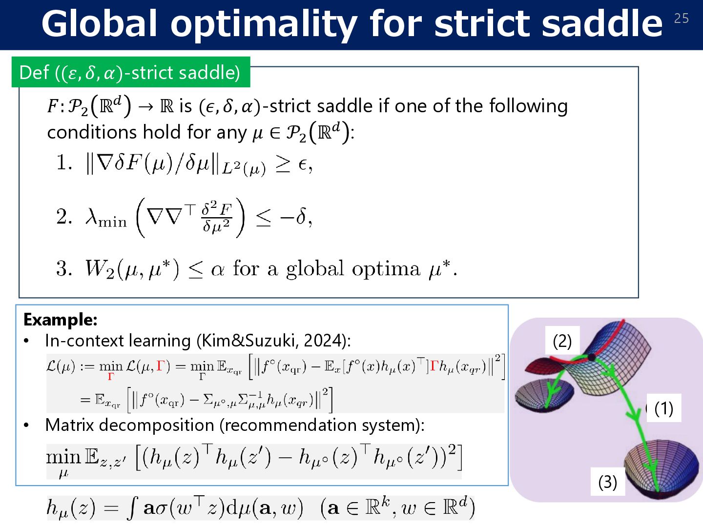
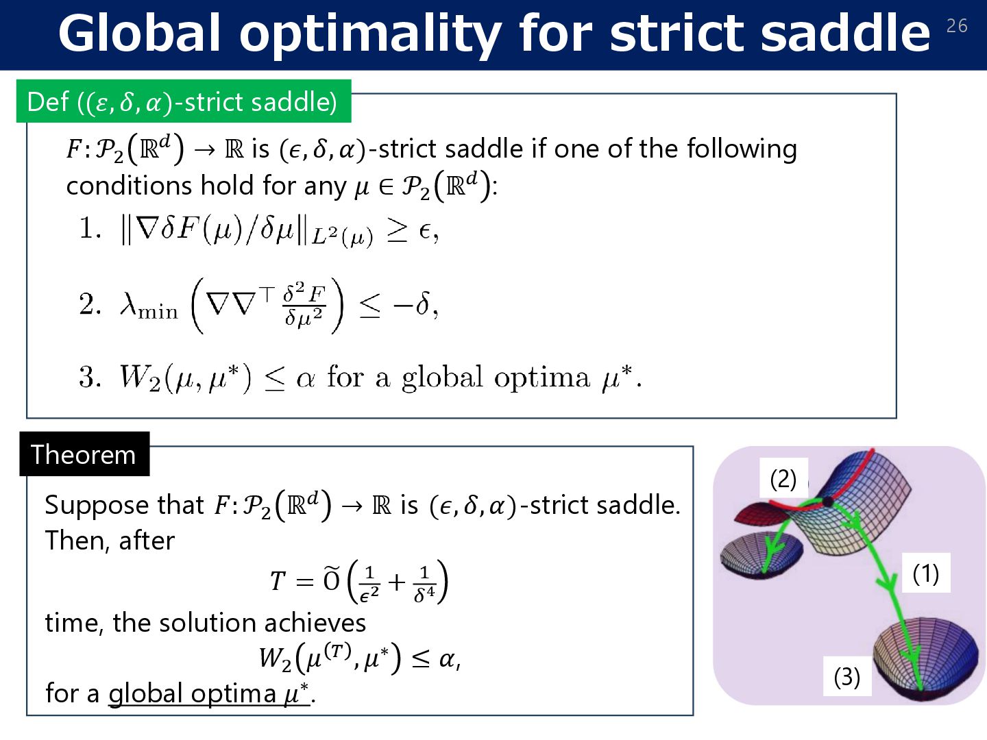
ℝ is (𝜖, 𝛿, 𝛼)-strict saddle if one of the following conditions hold for any 𝜇 ∈ 𝒫2 ℝ𝑑 : Def ((𝜀, 𝛿, 𝛼)-strict saddle) (2) (1) (3) Example: • In-context learning (Kim&Suzuki, 2024): • Matrix decomposition (recommendation system):
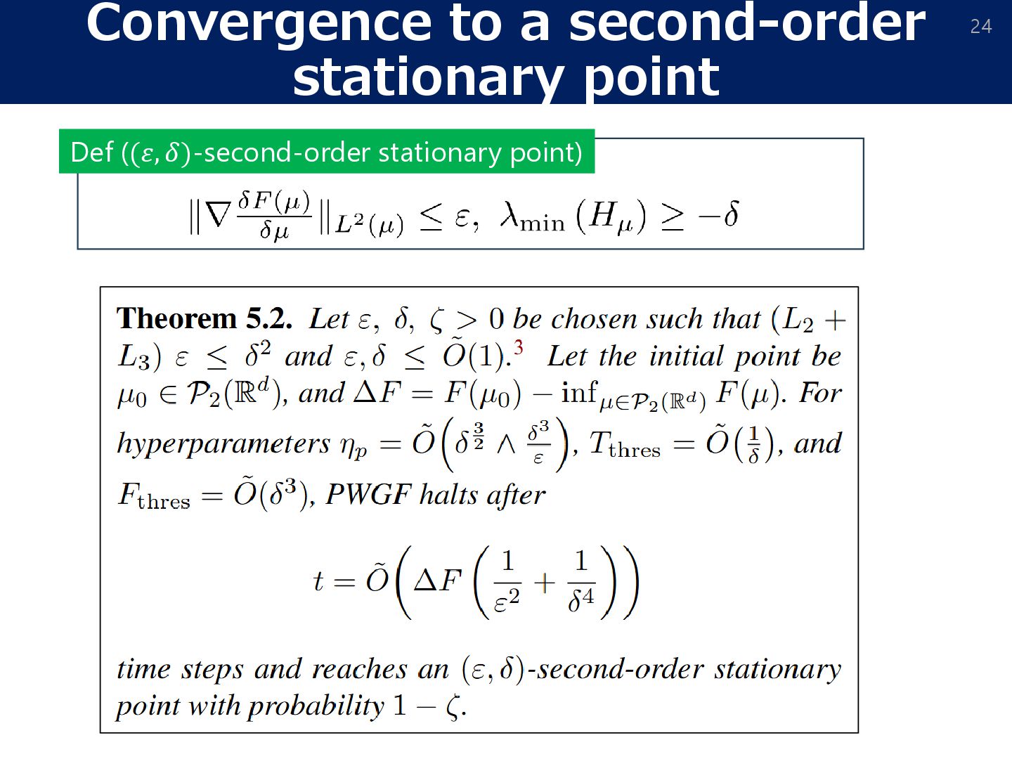
ℝ is (𝜖, 𝛿, 𝛼)-strict saddle if one of the following conditions hold for any 𝜇 ∈ 𝒫2 ℝ𝑑 : Def ((𝜀, 𝛿, 𝛼)-strict saddle) (2) (1) (3) Theorem Suppose that 𝐹: 𝒫2 ℝ𝑑 → ℝ is (𝜖, 𝛿, 𝛼)-strict saddle. Then, after 𝑇 = ෩ O 1 𝜖2 + 1 𝛿4 time, the solution achieves 𝑊2 𝜇 𝑇 , 𝜇∗ ≤ 𝛼, for a global optima 𝜇∗.
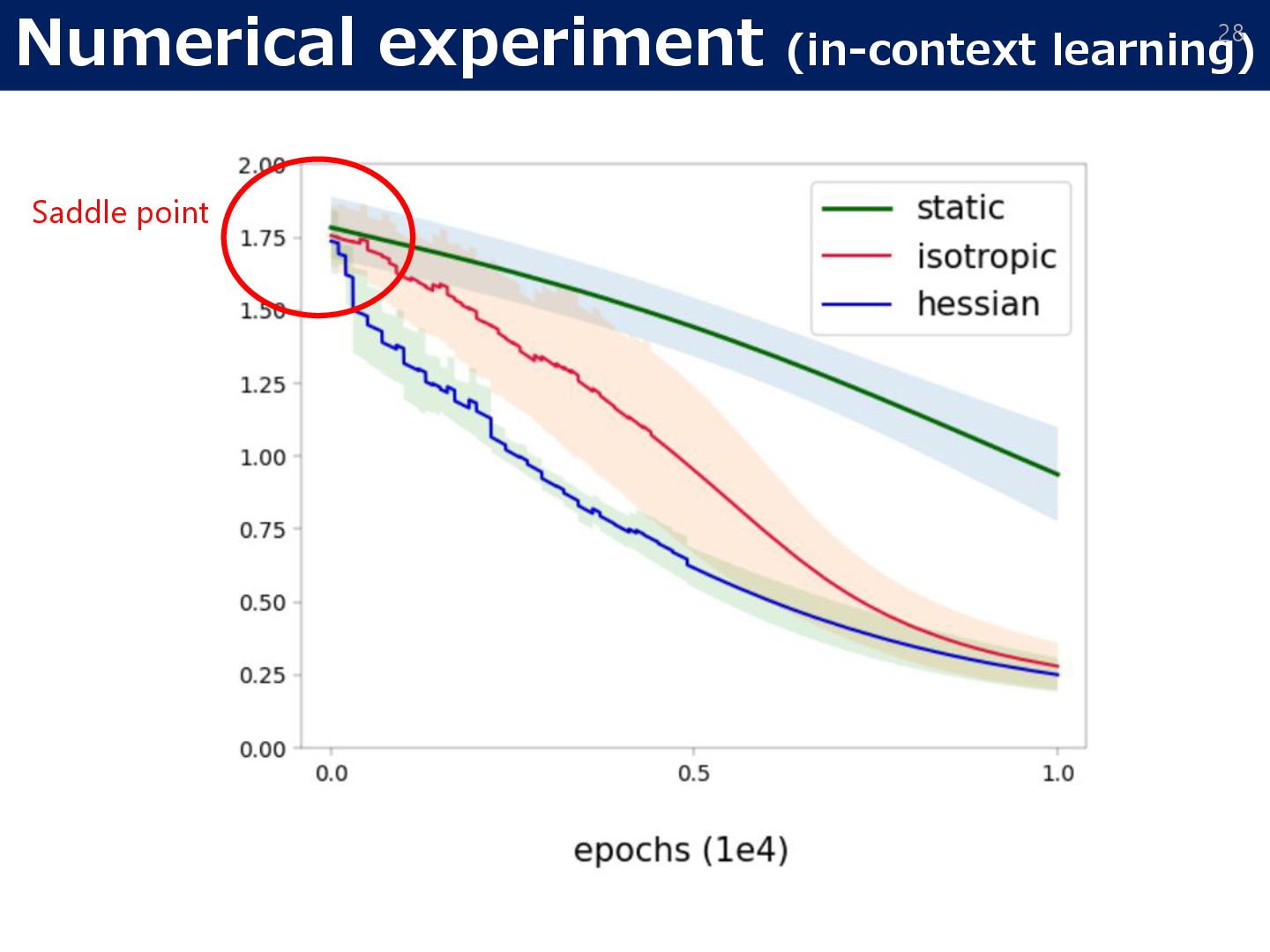
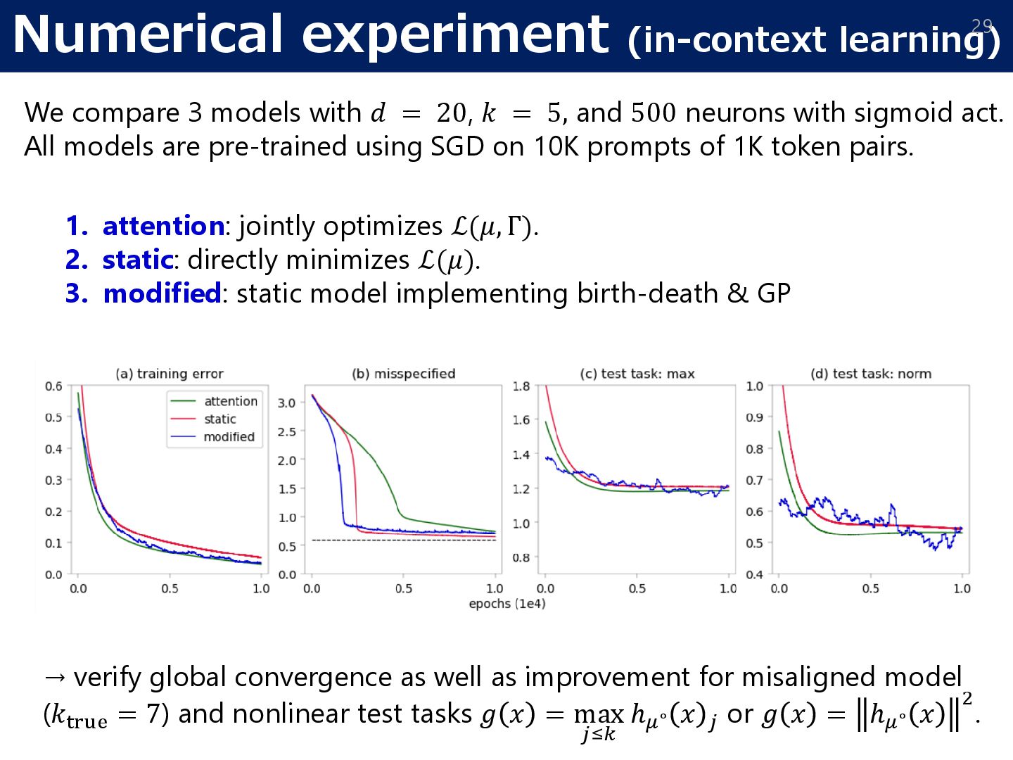
𝑑 = 20, 𝑘 = 5, and 500 neurons with sigmoid act. All models are pre-trained using SGD on 10K prompts of 1K token pairs. 1. attention: jointly optimizes ℒ(𝜇, Γ). 2. static: directly minimizes ℒ(𝜇). 3. modified: static model implementing birth-death & GP → verify global convergence as well as improvement for misaligned model (𝑘true = 7) and nonlinear test tasks 𝑔 𝑥 = max 𝑗≤𝑘 ℎ𝜇∘ 𝑥 𝑗 or 𝑔 𝑥 = ℎ𝜇∘ 𝑥 2 .
Sakaguchi, Suzuki: Propagation of Chaos for Mean-Field Langevin Dynamics and its Application to Model Ensemble. ICML2025. • [Optimization of a probability measure on a strict saddle objecive] - Kim, Suzuki: Transformers Learn Nonlinear Features In Context: Nonconvex Mean-field Dynamics on the Attention Landscape. ICML2024, oral. - Yamamto, Kim, Suzuki: Hessian-guided Perturbed Wasserstein Gradient Flows for Escaping Saddle Points. 2025. Part 2: Non-convex (strict-saddle objective) 1. Gaussian process perturbation: A polynomial time method to avoid a saddle point by a “random perturbation” of a probability measure. 2. In-context learning: The objective to train a two-layer transformer is strict-saddle. Mean-field Langevin dynamics (𝐹 𝜇 + 𝜆Ent(𝜇)) • Optimization of probability measures by WG-flow • Particle approximation • Defective log-Sobolev inequality Part 1: Convex (propagation of chaos)
![Presentation overview 3 • [Propagation of chaos] Nitanda, Lee, Kai,](https://files.speakerdeck.com/presentations/f449941225424ace8c2298b1468693f4/slide_2.jpg)
![Presentation overview 30 • [Propagation of chaos] Nitanda, Lee, Kai,](https://files.speakerdeck.com/presentations/f449941225424ace8c2298b1468693f4/slide_29.jpg)