Information Retrieval and Text Mining 2020 - Retrieval Models

University of Stavanger, DAT640, 2020 fall

Transcript

1. Retrieval Models [DAT640] Informa on Retrieval and Text Mining Krisz an Balog University of Stavanger September 28, 2020 CC BY 4.0
2. So far • Document retrieval task: scoring documents against a search query • Inverted index: special data structure to facilitate large-scale retrieval • Evaluation: measuring the goodness of a ranking against the ground truth using binary or graded relevance 2 / 49
3. Outline • Search engine architecture • Indexing and query processing • Evaluation • Retrieval models ⇐ this lecture • Query modeling • Web search • Semantic search • Learning-to-rank • Neural IR 3 / 49
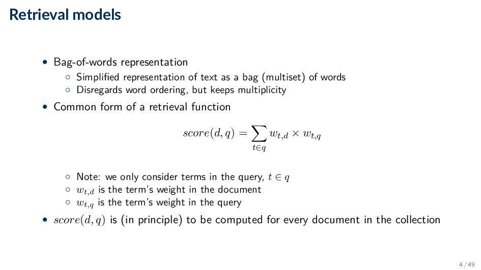
4. Retrieval models • Bag-of-words representation ◦ Simplified representation of text as a bag (multiset) of words ◦ Disregards word ordering, but keeps multiplicity • Common form of a retrieval function score(d, q) = t∈q wt,d × wt,q ◦ Note: we only consider terms in the query, t ∈ q ◦ wt,d is the term’s weight in the document ◦ wt,q is the term’s weight in the query • score(d, q) is (in principle) to be computed for every document in the collection 4 / 49
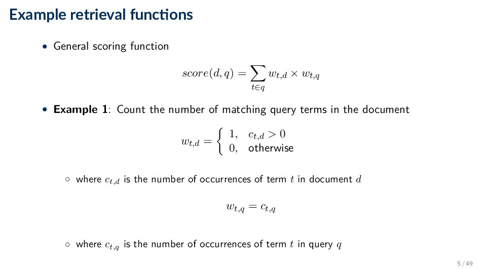
5. Example retrieval func ons • General scoring function score(d, q) = t∈q wt,d × wt,q • Example 1: Count the number of matching query terms in the document wt,d = 1, ct,d > 0 0, otherwise ◦ where ct,d is the number of occurrences of term t in document d wt,q = ct,q ◦ where ct,q is the number of occurrences of term t in query q 5 / 49
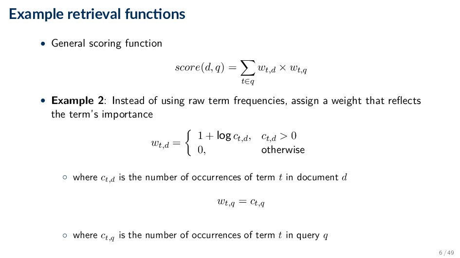
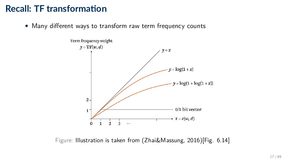
6. Example retrieval func ons • General scoring function score(d, q) = t∈q wt,d × wt,q • Example 2: Instead of using raw term frequencies, assign a weight that reflects the term’s importance wt,d = 1 + log ct,d, ct,d > 0 0, otherwise ◦ where ct,d is the number of occurrences of term t in document d wt,q = ct,q ◦ where ct,q is the number of occurrences of term t in query q 6 / 49
7. Vector Space Model 7 / 49
8. Vector space model • Basis of most IR research in the 1960s and 70s • Still used • Provides a simple and intuitively appealing framework for implementing ◦ Term weighting ◦ Ranking ◦ Relevance feedback 8 / 49
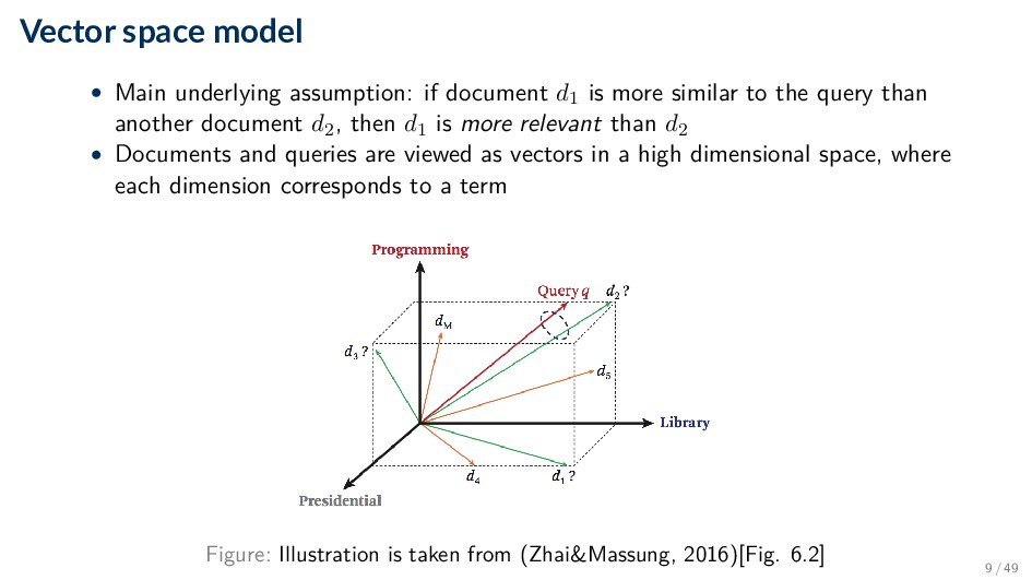
9. Vector space model • Main underlying assumption: if document d1 is more similar to the query than another document d2, then d1 is more relevant than d2 • Documents and queries are viewed as vectors in a high dimensional space, where each dimension corresponds to a term Figure: Illustration is taken from (Zhai&Massung, 2016)[Fig. 6.2] 9 / 49
10. Instan a on • The vector space model provides a framework that needs to be instantiated by deciding ◦ How to select terms? (i.e., vocabulary construction) ◦ How to place documents and queries in the vector space (i.e., term weighting) ◦ How to measure the similarity between two vectors (i.e., similarity measure) 10 / 49
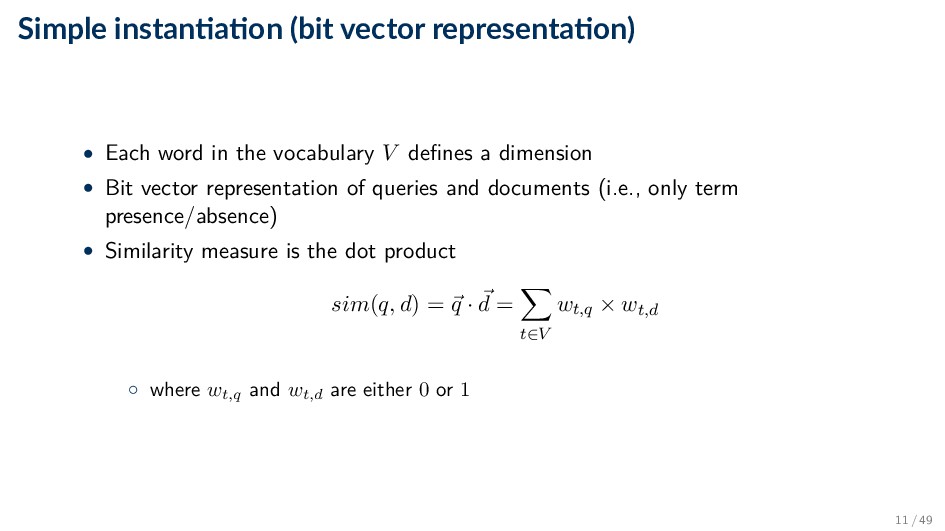
11. Simple instan a on (bit vector representa on) • Each word in the vocabulary V defines a dimension • Bit vector representation of queries and documents (i.e., only term presence/absence) • Similarity measure is the dot product sim(q, d) = q · d = t∈V wt,q × wt,d ◦ where wt,q and wt,d are either 0 or 1 11 / 49
12. Discussion Question What are potential shortcomings of this simple instantiation? 12 / 49
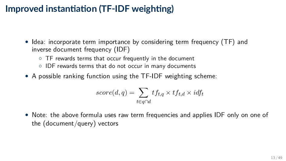
13. Improved instan a on (TF-IDF weigh ng) • Idea: incorporate term importance by considering term frequency (TF) and inverse document frequency (IDF) ◦ TF rewards terms that occur frequently in the document ◦ IDF rewards terms that do not occur in many documents • A possible ranking function using the TF-IDF weighting scheme: score(d, q) = t∈q∩d tft,q × tft,d × idft • Note: the above formula uses raw term frequencies and applies IDF only on one of the (document/query) vectors 13 / 49
14. Many different variants out there! • Different variants of TF and IDF • Different TF-IDF weighting for the query and for the document • Different similarity measure (e.g., cosine) 14 / 49
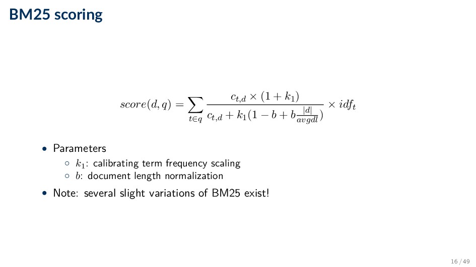
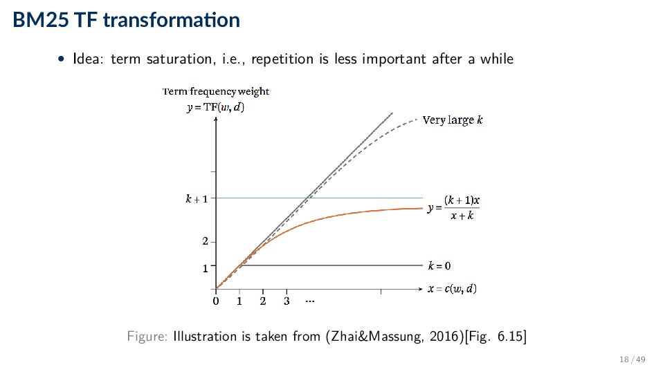
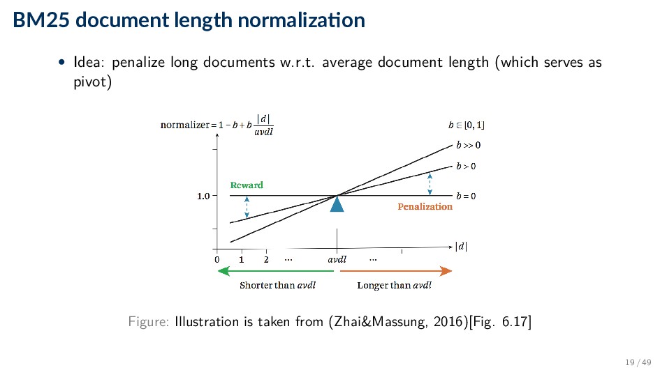
15. BM25 • BM25 was created as the result of a series of experiments (“Best Match”) • Popular and effective ranking algorithm • The reasoning behind BM25 is that good term weighting is based on three principles ◦ Term frequency ◦ Inverse document frequency ◦ Document length normalization 15 / 49
16. BM25 scoring score(d, q) = t∈q ct,d × (1 + k1) ct,d + k1(1 − b + b |d| avgdl ) × idft • Parameters ◦ k1 : calibrating term frequency scaling ◦ b: document length normalization • Note: several slight variations of BM25 exist! 16 / 49
17. Recall: TF transforma on • Many different ways to transform raw term frequency counts Figure: Illustration is taken from (Zhai&Massung, 2016)[Fig. 6.14] 17 / 49
18. BM25 TF transforma on • Idea: term saturation, i.e., repetition is less important after a while Figure: Illustration is taken from (Zhai&Massung, 2016)[Fig. 6.15] 18 / 49
19. BM25 document length normaliza on • Idea: penalize long documents w.r.t. average document length (which serves as pivot) Figure: Illustration is taken from (Zhai&Massung, 2016)[Fig. 6.17] 19 / 49
20. BM25 parameter se ng • k1: calibrating term frequency scaling ◦ 0 corresponds to a binary model ◦ large values correspond to using raw term frequencies ◦ typical values are between 1.2 and 2.0; a common default value is 1.2 • b: document length normalization ◦ 0: no normalization at all ◦ 1: full length normalization ◦ typical value: 0.75 20 / 49
21. Language Models 21 / 49
22. Language models • Based on the notion of probabilities and processes for generating text • Wide range of usage across different applications ◦ Speech recognition • “I ate a cherry” is a more likely sentence than “Eye eight uh Jerry” ◦ OCR and handwriting recognition • More probable sentences are more likely correct readings ◦ Machine translation • More likely sentences are probably better translations 22 / 49
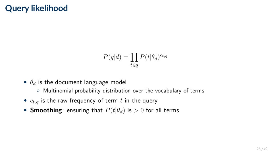
23. Language models for ranking documents • Represent each document as a multinomial probability distribution over terms • Estimate the probability that the query was “generated” by the given document ◦ How likely is the search query given the language model of the document? 23 / 49
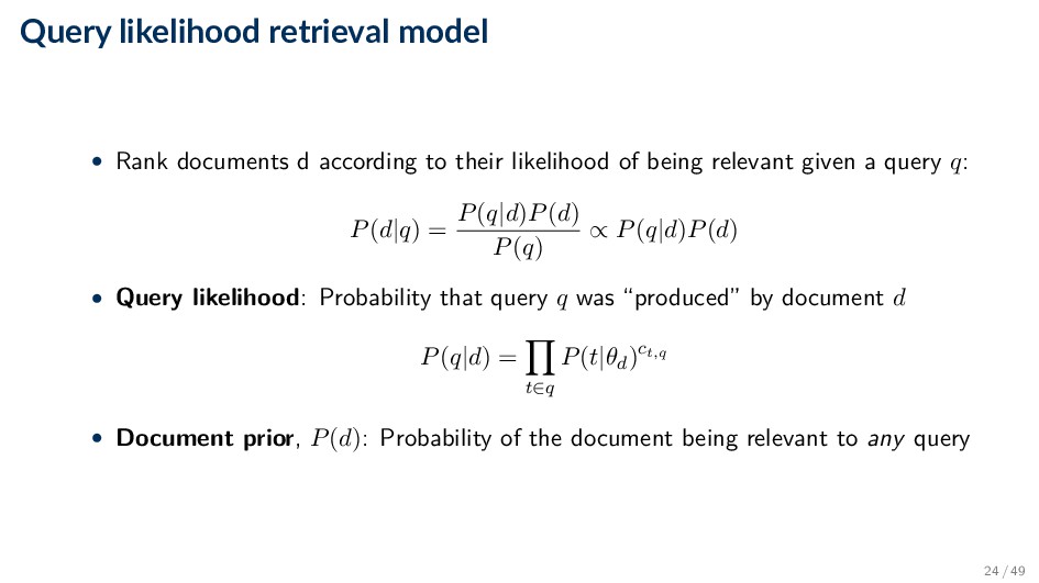
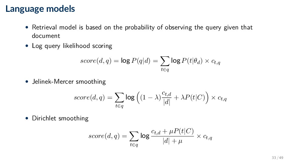
24. Query likelihood retrieval model • Rank documents d according to their likelihood of being relevant given a query q: P(d|q) = P(q|d)P(d) P(q) ∝ P(q|d)P(d) • Query likelihood: Probability that query q was “produced” by document d P(q|d) = t∈q P(t|θd)ct,q • Document prior, P(d): Probability of the document being relevant to any query 24 / 49
25. Query likelihood P(q|d) = t∈q P(t|θd)ct,q • θd is the document language model ◦ Multinomial probability distribution over the vocabulary of terms • ct,q is the raw frequency of term t in the query • Smoothing: ensuring that P(t|θd) is > 0 for all terms 25 / 49
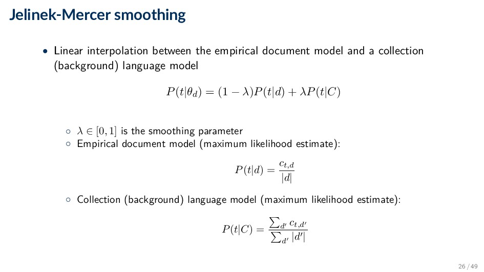
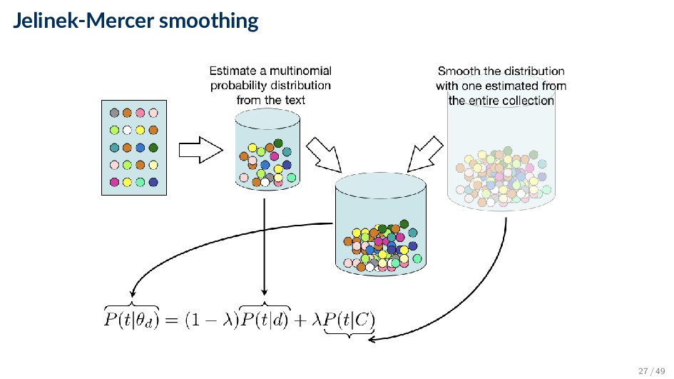
26. Jelinek-Mercer smoothing • Linear interpolation between the empirical document model and a collection (background) language model P(t|θd) = (1 − λ)P(t|d) + λP(t|C) ◦ λ ∈ [0, 1] is the smoothing parameter ◦ Empirical document model (maximum likelihood estimate): P(t|d) = ct,d |d| ◦ Collection (background) language model (maximum likelihood estimate): P(t|C) = d ct,d d |d | 26 / 49
27. Jelinek-Mercer smoothing 27 / 49
28. Dirichlet smoothing • Smoothing is inversely proportional to the document length P(t|θd) = ct,d + µP(t|C) |d| + µ ◦ µ is the smoothing parameter (typically ranges from 10 to 10000) • Notice that Dirichlet smoothing may also be viewed as a linear interpolation in the style of Jelinek-Mercer smoothing, by setting λ = µ |d| + µ (1 − λ) = |d| |d| + µ 28 / 49
29. Query likelihood scoring (Example) • query: “sea submarine” P(q|d) = P(sea|θd) × P(submarine|θd) = (1 − λ)P(sea|d) + λP(sea|C) × (1 − λ)P(submarine|d) + λP(submarine|C) • where ◦ P(sea|d) is the relative frequency of term “sea” in document d ◦ P(sea|C) is the relative frequency of term “sea” in the entire collection ◦ ... 29 / 49
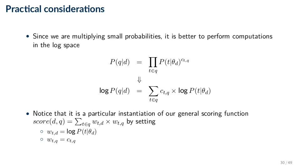
30. Prac cal considera ons • Since we are multiplying small probabilities, it is better to perform computations in the log space P(q|d) = t∈q P(t|θd)ct,q ⇓ log P(q|d) = t∈q ct,q × log P(t|θd) • Notice that it is a particular instantiation of our general scoring function score(d, q) = t∈q wt,d × wt,q by setting ◦ wt,d = log P(t|θd ) ◦ wt,q = ct,q 30 / 49
31. Summary 31 / 49
32. BM25 • Retrieval model is based on the idea of query-document similarity. Three main components: ◦ Term frequency ◦ Inverse document frequency ◦ Document length normalization • Retrieval function score(d, q) = t∈q ct,d × (1 + k1) ct,d + k1(1 − b + b |d| avgdl ) × idft ◦ Parameters • k1 : calibrating term frequency scaling (k1 ∈ [1.2..2]) • b: document length normalization (b ∈ [0, 1]) 32 / 49
33. Language models • Retrieval model is based on the probability of observing the query given that document • Log query likelihood scoring score(d, q) = log P(q|d) = t∈q log P(t|θd) × ct,q • Jelinek-Mercer smoothing score(d, q) = t∈q log (1 − λ) ct,d |d| + λP(t|C) × ct,q • Dirichlet smoothing score(d, q) = t∈q log ct,d + µP(t|C) |d| + µ × ct,q 33 / 49
34. Discussion Question What other statistics are needed to compute these retrieval functions, in addition to term frequencies (ct,d)? 34 / 49
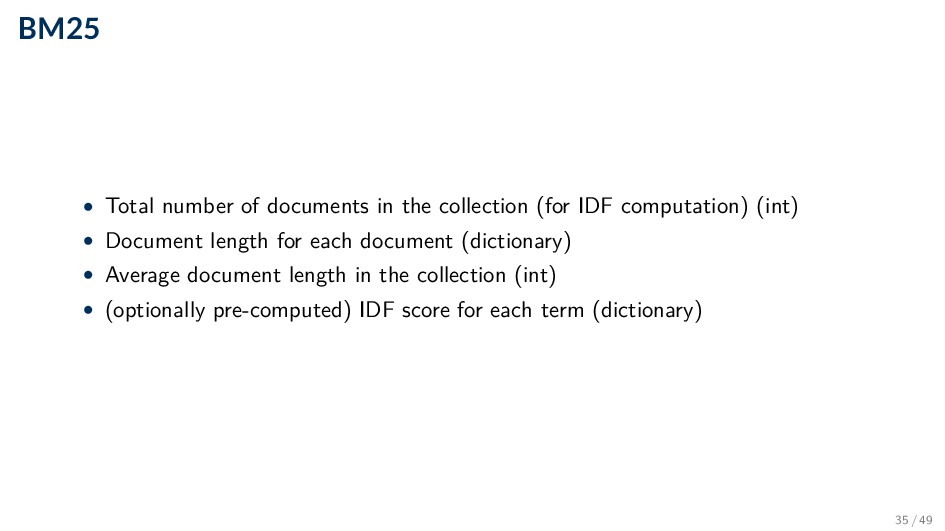
35. BM25 • Total number of documents in the collection (for IDF computation) (int) • Document length for each document (dictionary) • Average document length in the collection (int) • (optionally pre-computed) IDF score for each term (dictionary) 35 / 49
36. Language models • Document length for each document (dictionary) • Sum TF for each term (dictionary) • Sum of all document lengths in the collection (int) • (optionally pre-computed) Collection term probability P(t|C) for each term (dictionary) 36 / 49
37. Fielded (variants of) Retrieval Models 37 / 49
38. Mo va on • Documents are composed of multiple fields ◦ E.g., title, body, anchors, etc. • Modeling internal document structure may be beneficial for retrieval 38 / 49
39. Example 39 / 49
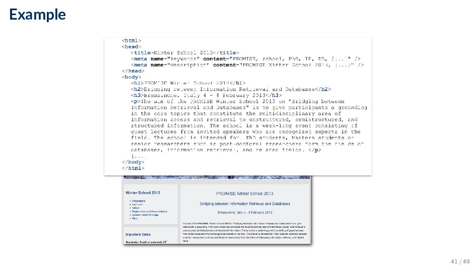
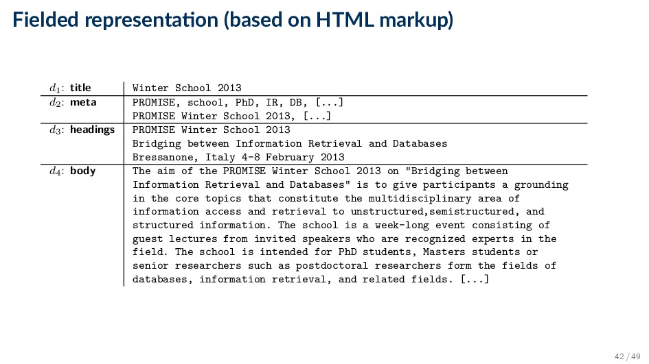
40. Unstructured representa on PROMISE Winter School 2013 Bridging between Information Retrieval and Databases Bressanone, Italy 4 - 8 February 2013 The aim of the PROMISE Winter School 2013 on "Bridging between Information Retrieval and Databases" is to give participants a grounding in the core topics that constitute the multidisciplinary area of information access and retrieval to unstructured, semistructured, and structured information. The school is a week-long event consisting of guest lectures from invited speakers who are recognized experts in the field. The school is intended for PhD students, Masters students or senior researchers such as post-doctoral researchers form the fields of databases, information retrieval, and related fields. [...] 40 / 49
41. Example 41 / 49
42. Fielded representa on (based on HTML markup) d1: title Winter School 2013 d2: meta PROMISE, school, PhD, IR, DB, [...] PROMISE Winter School 2013, [...] d3: headings PROMISE Winter School 2013 Bridging between Information Retrieval and Databases Bressanone, Italy 4-8 February 2013 d4: body The aim of the PROMISE Winter School 2013 on "Bridging between Information Retrieval and Databases" is to give participants a grounding in the core topics that constitute the multidisciplinary area of information access and retrieval to unstructured,semistructured, and structured information. The school is a week-long event consisting of guest lectures from invited speakers who are recognized experts in the field. The school is intended for PhD students, Masters students or senior researchers such as postdoctoral researchers form the fields of databases, information retrieval, and related fields. [...] 42 / 49
43. Fielded extension of retrieval models • BM25 ⇒ BM25F • Language Models (LM) ⇒ Mixture of Language Models (MLM) 43 / 49
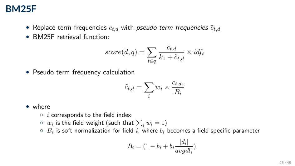
44. BM25F • Extension of BM25 incorporating multiple fields • The soft normalization and term frequencies need to be adjusted • Original BM25 retrieval function: score(d, q) = t∈q ct,d × (1 + k1) ct,d + k1 × B × idft • where B is is the soft normalization: B = (1 − b + b |d| avgdl ) 44 / 49
45. BM25F • Replace term frequencies ct,d with pseudo term frequencies ˜ ct,d • BM25F retrieval function: score(d, q) = t∈q ˜ ct,d k1 + ˜ ct,d × idft • Pseudo term frequency calculation ˜ ct,d = i wi × ct,di Bi • where ◦ i corresponds to the field index ◦ wi is the field weight (such that i wi = 1) ◦ Bi is soft normalization for field i, where bi becomes a field-specific parameter Bi = (1 − bi + bi |di | avgdli ) 45 / 49
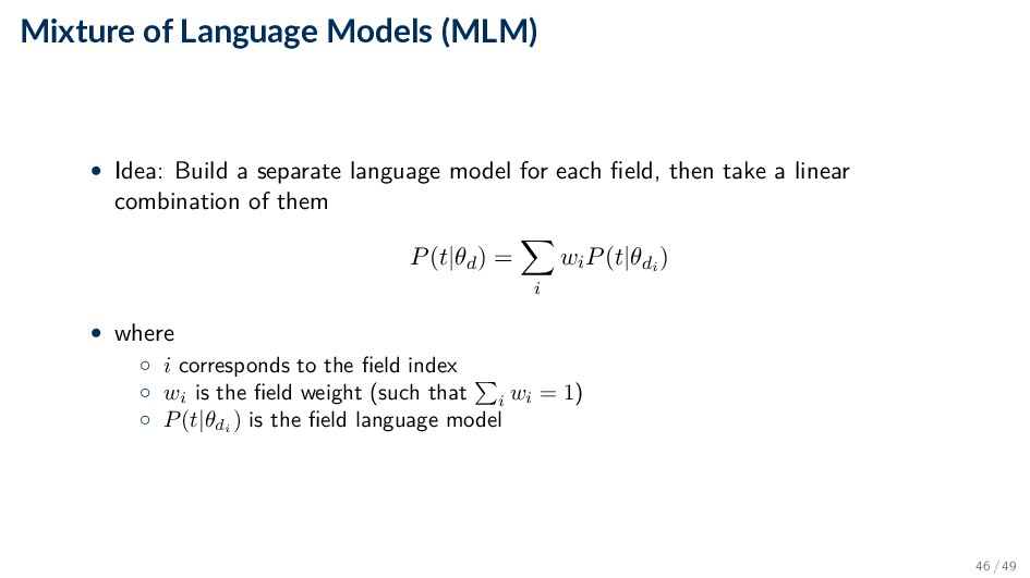
46. Mixture of Language Models (MLM) • Idea: Build a separate language model for each field, then take a linear combination of them P(t|θd) = i wiP(t|θdi ) • where ◦ i corresponds to the field index ◦ wi is the field weight (such that i wi = 1) ◦ P(t|θdi ) is the field language model 46 / 49
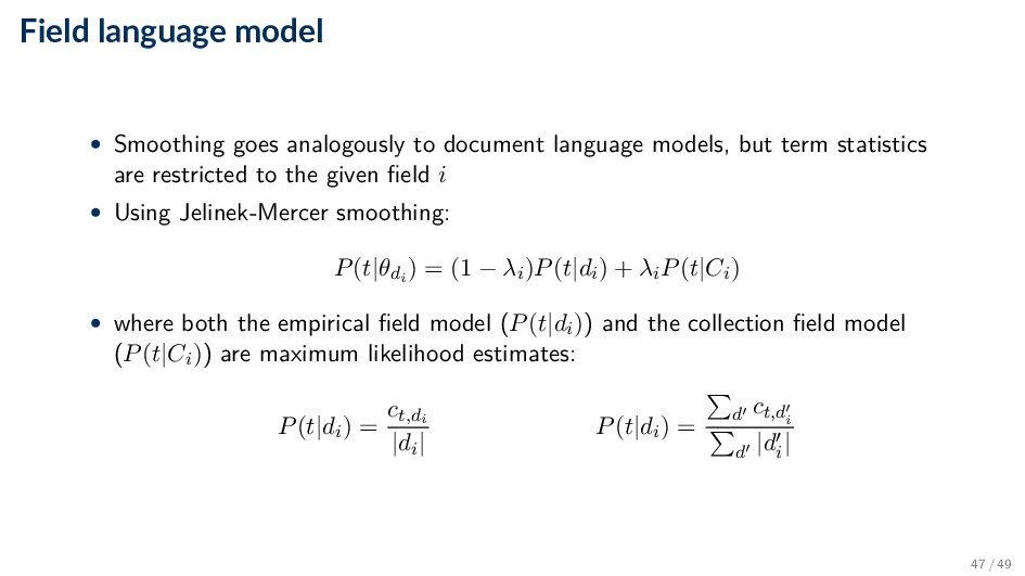
47. Field language model • Smoothing goes analogously to document language models, but term statistics are restricted to the given field i • Using Jelinek-Mercer smoothing: P(t|θdi ) = (1 − λi)P(t|di) + λiP(t|Ci) • where both the empirical field model (P(t|di)) and the collection field model (P(t|Ci)) are maximum likelihood estimates: P(t|di) = ct,di |di| P(t|di) = d ct,d i d |di | 47 / 49
48. Se ng parameter values • Retrieval models often contain parameters that must be tuned to get the best performance for specific types of data and queries • For experiments ◦ Use training and test data sets ◦ If less data available, use cross-validation by partitioning the data into k subsets • Many techniques exist to find optimal parameter values given training data ◦ Standard problem in machine learning • For standard retrieval models, involving few parameters, grid search is feasible ◦ Perform a sweep over the possible values of each parameter, e.g., from 0 to 1 in steps of 0.1 48 / 49
49. Reading • Text Data Management and Analysis (Zhai&Massung) ◦ Chapter 6 49 / 49