Information Retrieval and Text Mining - Text Classification (Part III)

University of Stavanger, DAT640, 2019 fall

Transcript

1. Text Classifica on (Part III) [DAT640] Informa on Retrieval and Text Mining Krisz an Balog University of Stavanger August 27, 2019
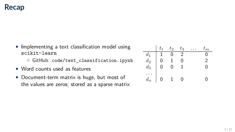
2. Recap • Implementing a text classification model using scikit-learn ◦ GitHub: code/text_classification.ipynb • Word counts used as features • Document-term matrix is huge, but most of the values are zeros; stored as a sparse matrix t1 t2 t3 . . . tm d1 1 0 2 0 d2 0 1 0 2 d3 0 0 1 0 . . . dn 0 1 0 0 2 / 15
3. Discussion Question What are possible shortcomings of using raw term frequencies? 3 / 15
4. Zip’s law • Given some corpus of natural language utterances, the frequency of any word is inversely proportional to its rank in the frequency table ◦ Word number n has a frequency proportional to 1/n 4 / 15
5. English language • Most frequent words ◦ the (7%) ◦ of (3.5%) ◦ and (2.8%) • Top 135 most frequent words account for half of the words used 5 / 15
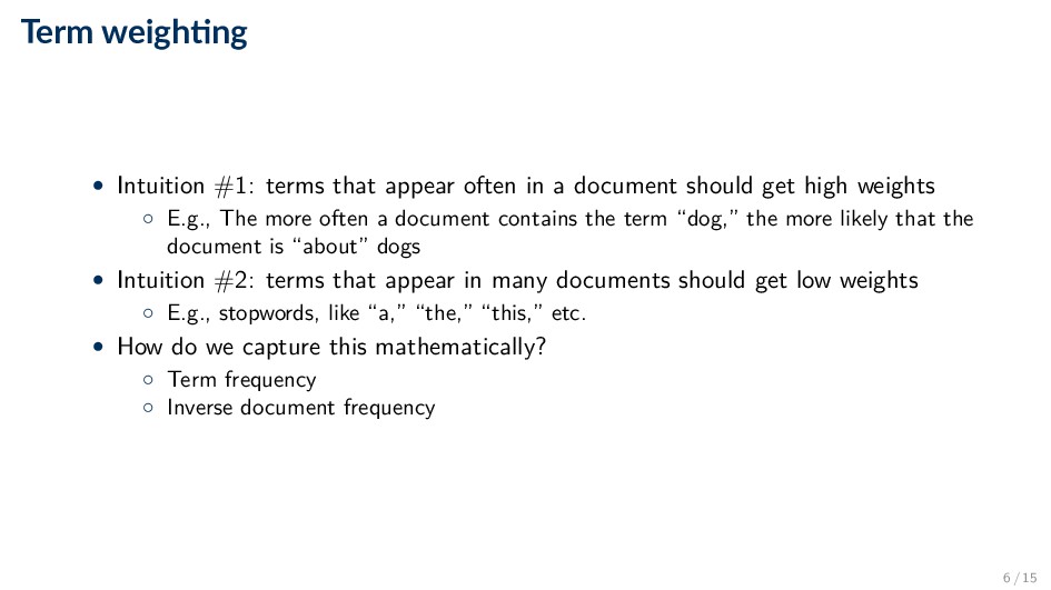
6. Term weigh ng • Intuition #1: terms that appear often in a document should get high weights ◦ E.g., The more often a document contains the term “dog,” the more likely that the document is “about” dogs • Intuition #2: terms that appear in many documents should get low weights ◦ E.g., stopwords, like “a,” “the,” “this,” etc. • How do we capture this mathematically? ◦ Term frequency ◦ Inverse document frequency 6 / 15
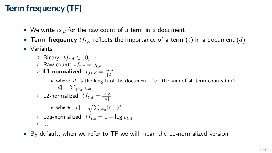
7. Term frequency (TF) • We write ct,d for the raw count of a term in a document • Term frequency tft,d reflects the importance of a term (t) in a document (d) • Variants ◦ Binary: tft,d ∈ {0, 1} ◦ Raw count: tft,d = ct,d ◦ L1-normalized: tft,d = ct,d |d| • where |d| is the length of the document, i.e., the sum of all term counts in d: |d| = t∈d ct,d ◦ L2-normalized: tft,d = ct,d ||d|| • where ||d|| = t∈d (ct,d )2 ◦ Log-normalized: tft,d = 1 + log ct,d ◦ ... • By default, when we refer to TF we will mean the L1-normalized version 7 / 15
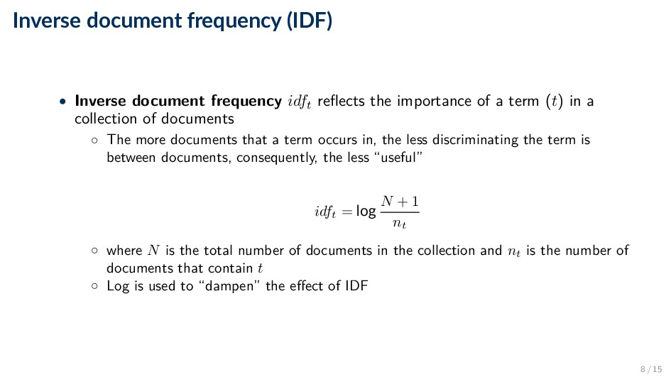
8. Inverse document frequency (IDF) • Inverse document frequency idft reflects the importance of a term (t) in a collection of documents ◦ The more documents that a term occurs in, the less discriminating the term is between documents, consequently, the less “useful” idft = log N + 1 nt ◦ where N is the total number of documents in the collection and nt is the number of documents that contain t ◦ Log is used to “dampen” the effect of IDF 8 / 15
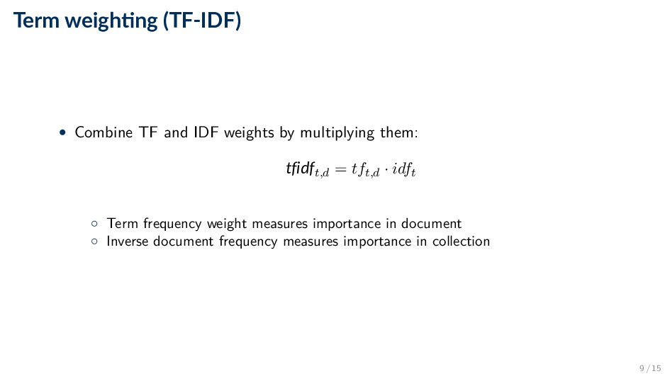
9. Term weigh ng (TF-IDF) • Combine TF and IDF weights by multiplying them: tfidft,d = tft,d · idft ◦ Term frequency weight measures importance in document ◦ Inverse document frequency measures importance in collection 9 / 15
10. Exercise #1 (paper-based) Create document-term matrix using TF-IDF weighting from a set of documents. 10 / 15
11. Code • GitHub: code/text_feature_extraction.ipynb 11 / 15
12. Text classifica on training data (documents with known category labels) test data (documents without category labels) model learn model apply model 12 / 15
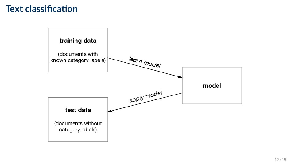
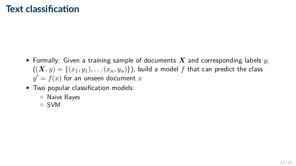
13. Text classifica on • Formally: Given a training sample of documents X and corresponding labels y, ((X, y) = {(x1, y1), . . . (xn, yn)}), build a model f that can predict the class y = f(x) for an unseen document x • Two popular classification models: ◦ Naive Bayes ◦ SVM 13 / 15
14. Exercise #2 (coding) • Compare two machine learning models and different term weighting schemes ◦ Naive Bayes and SVM ◦ Raw term count, TF weighting, and TF-IDF weighting • Complete the TODOs and fill out the results table GitHub: exercises/lecture_04/exercise_2.ipynb (make a local copy) 14 / 15
15. Assignment 1B 15 / 15