student passes the exam, based on his/her 7-day study hours prior to the exam. A hypothesis: a student will pass if he/she has studied for at least 15 hours
student passes the exam, based on his/her 7-day study hours prior to the exam. A hypothesis: a student will pass if he/she has studied for at least 15 hours We want to know if new incoming emails are of spam or not.
student passes the exam, based on his/her 7-day study hours prior to the exam. A hypothesis: a student will pass if he/she has studied for at least 15 hours We want to know if new incoming emails are of spam or not. A hypothesis: if an email contains words ”selamat” and ”hadiah”, then it is a spam.
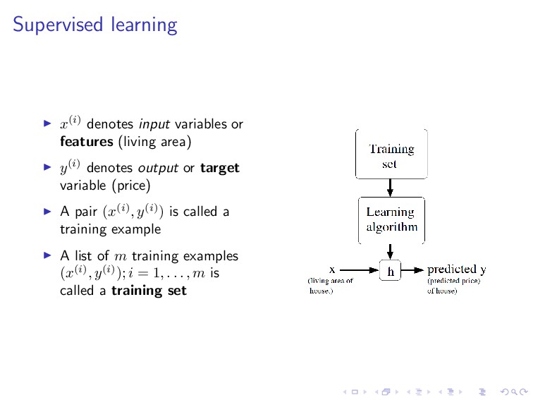
y(i) denotes output or target variable (price) A pair (x(i), y(i)) is called a training example A list of m training examples (x(i), y(i)); i = 1, . . . , m is called a training set
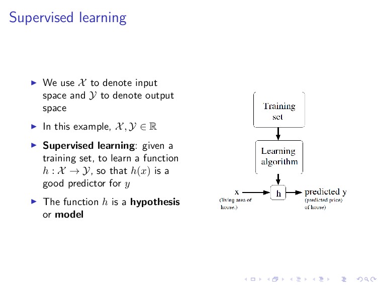
Y to denote output space In this example, X, Y ∈ R Supervised learning: given a training set, to learn a function h : X → Y, so that h(x) is a good predictor for y The function h is a hypothesis or model
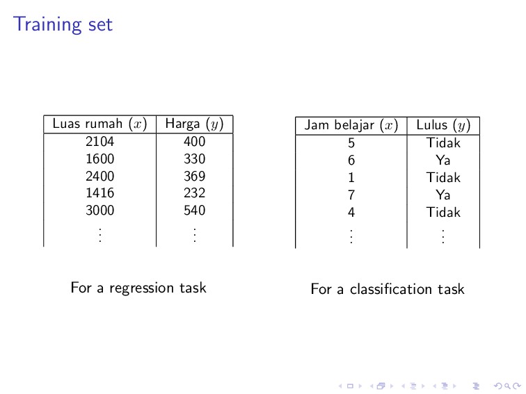
330 2400 369 1416 232 3000 540 . . . . . . For a regression task Jam belajar (x) Lulus (y) 5 Tidak 6 Ya 1 Tidak 7 Ya 4 Tidak . . . . . . For a classification task
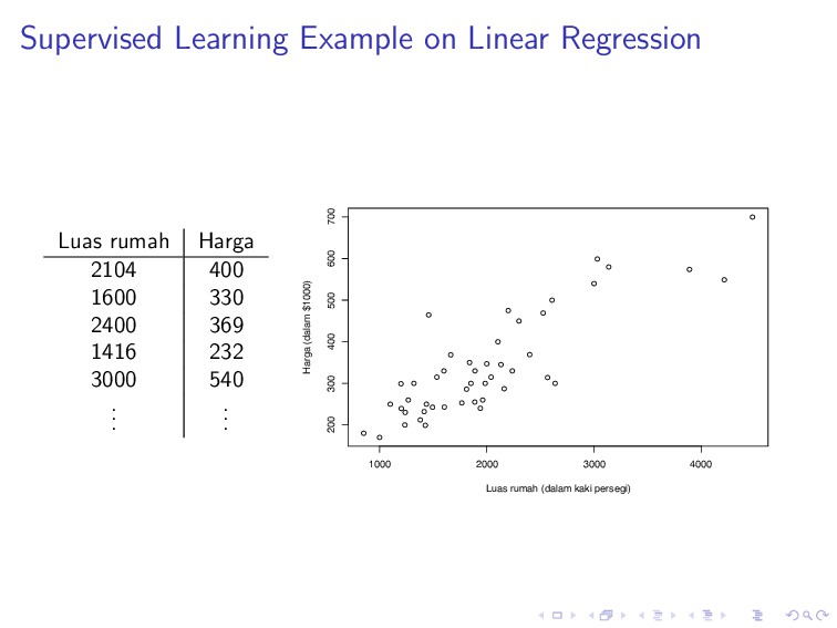
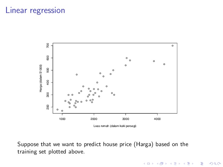
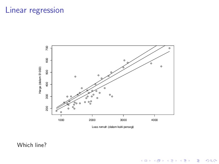
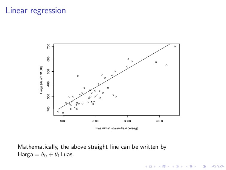
600 700 Luas rumah (dalam kaki persegi) Harga (dalam $1000) Suppose that we want to predict house price (Harga) based on the training set plotted above.
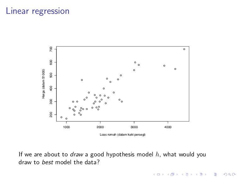
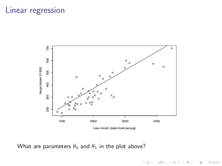
600 700 Luas rumah (dalam kaki persegi) Harga (dalam $1000) If we are about to draw a good hypothesis model h, what would you draw to best model the data?
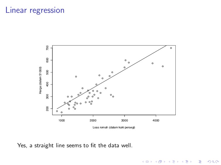
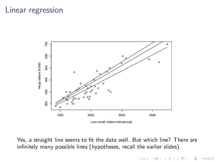
600 700 Luas rumah (dalam kaki persegi) Harga (dalam $1000) Yes, a straight line seems to fit the data well. But which line? There are infinitely many possible lines (hypotheses, recall the earlier slides).
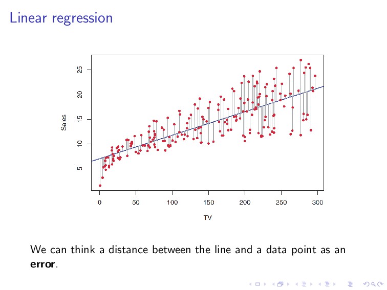
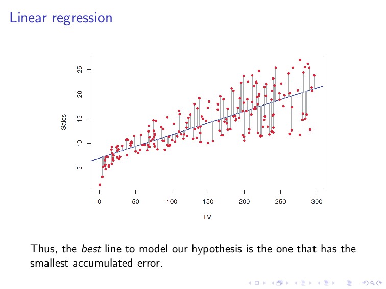
line that is approximately going through the middle of the data distribution. If we think in terms of distance, the best line is the one that is close to every data point.
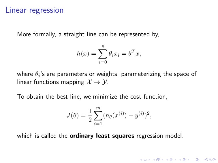
by, h(x) = n i=0 θixi = θT x, where θi’s are parameters or weights, parameterizing the space of linear functions mapping X → Y. To obtain the best line, we minimize the cost function, J(θ) = 1 2 m i=1 (hθ(x(i)) − y(i))2, which is called the ordinary least squares regression model.
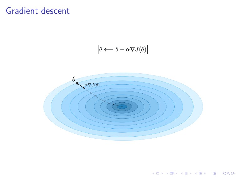
the gradient descent approach: 1. Pick an initial guess of θ 2. Repeatedly changes θ to make J(θ) smaller 3. Until hopefully converge to a value that minimizes J(θ)
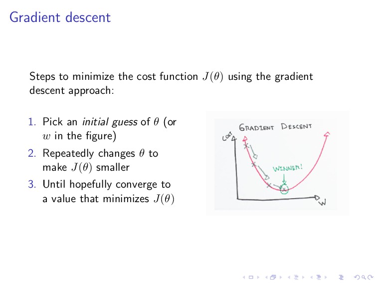
the gradient descent approach: 1. Pick an initial guess of θ (or w in the figure) 2. Repeatedly changes θ to make J(θ) smaller 3. Until hopefully converge to a value that minimizes J(θ)
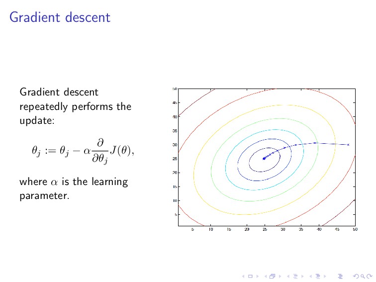
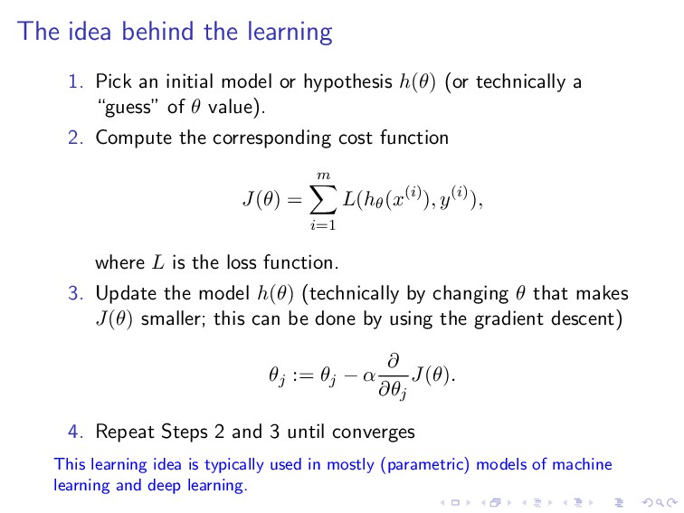
or hypothesis h(θ) (or technically a “guess” of θ value). 2. Compute the corresponding cost function J(θ) = m i=1 L(hθ(x(i)), y(i)), where L is the loss function. 3. Update the model h(θ) (technically by changing θ that makes J(θ) smaller; this can be done by using the gradient descent) θj := θj − α ∂ ∂θj J(θ). 4. Repeat Steps 2 and 3 until converges This learning idea is typically used in mostly (parametric) models of machine learning and deep learning.
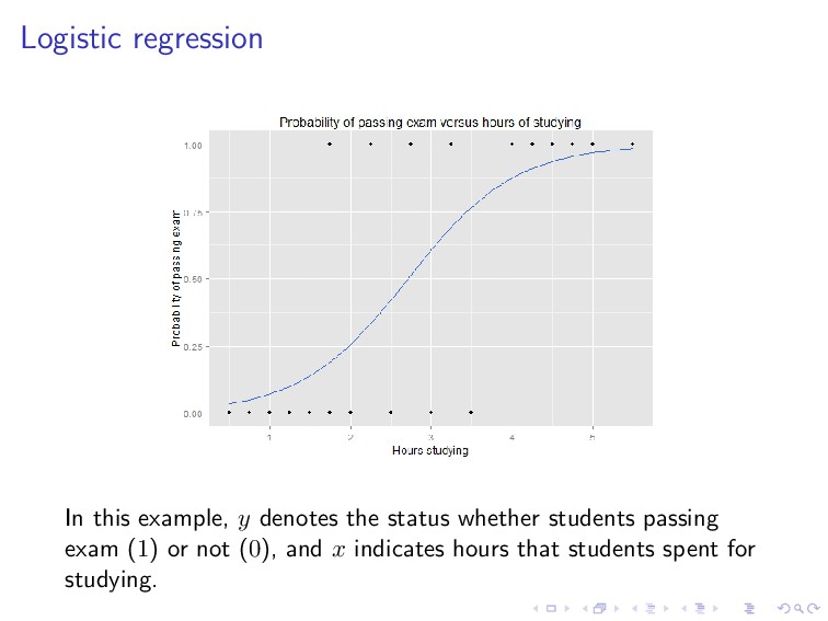
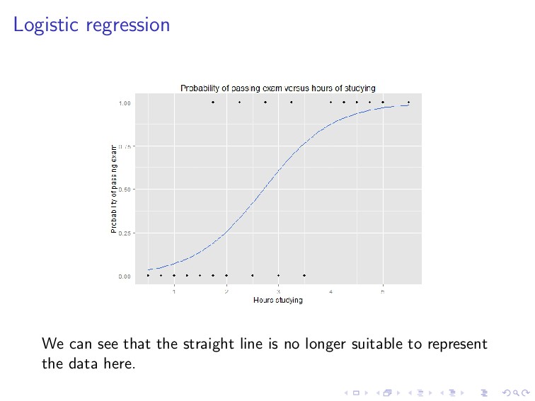
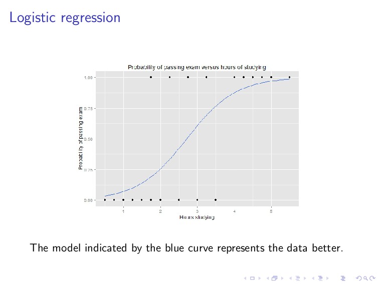
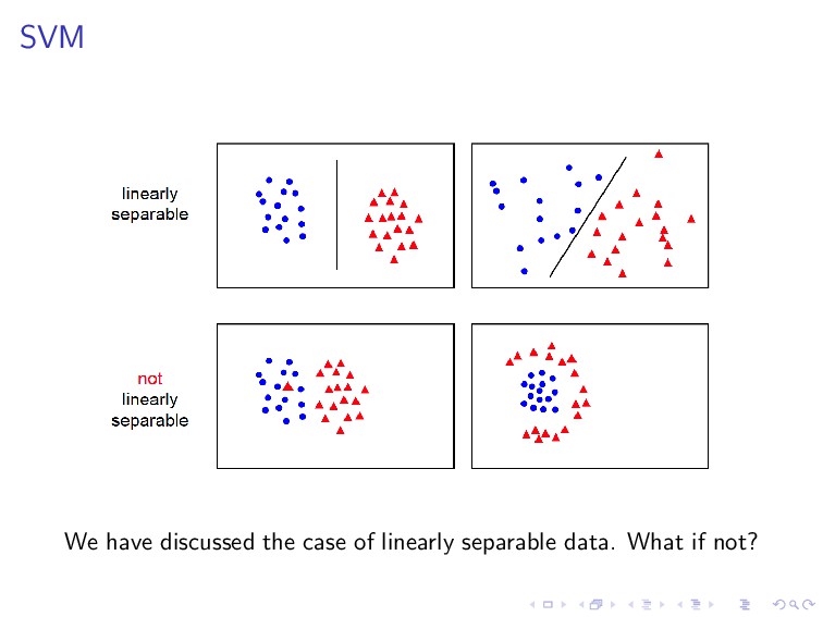
that y is continuous (e.g., house price). What if y is discrete? For example, if y indicates whether an email is a spam (1) or not (0), or whether a student passes the exam (1) or not (0). This problem is called classification.
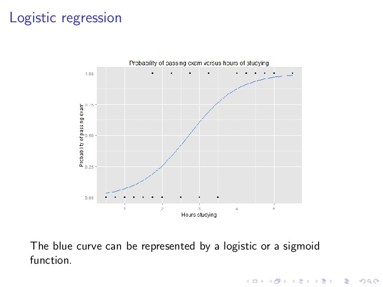
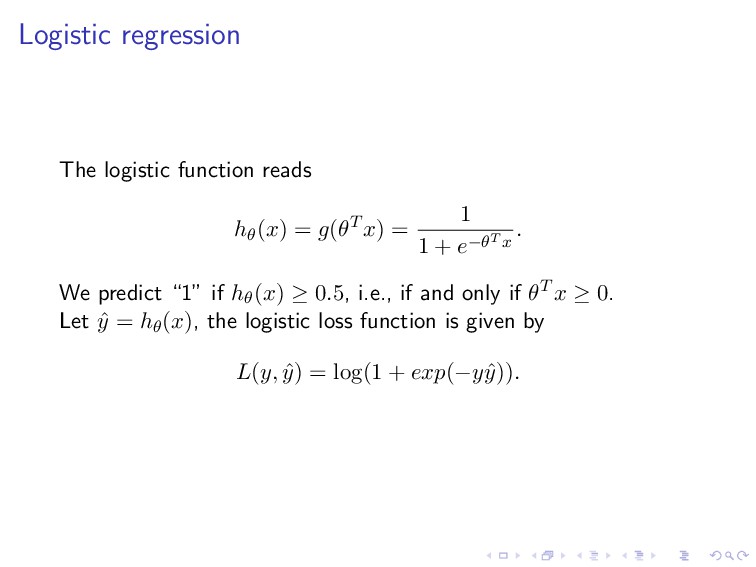
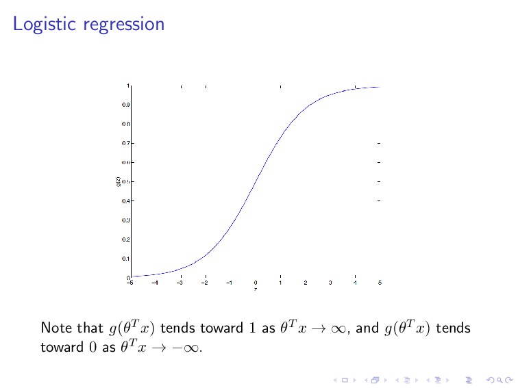
= 1 1 + e−θT x . We predict “1” if hθ(x) ≥ 0.5, i.e., if and only if θT x ≥ 0. Let ˆ y = hθ(x), the logistic loss function is given by L(y, ˆ y) = log(1 + exp(−yˆ y)).
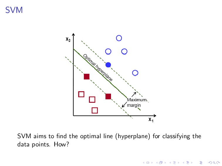
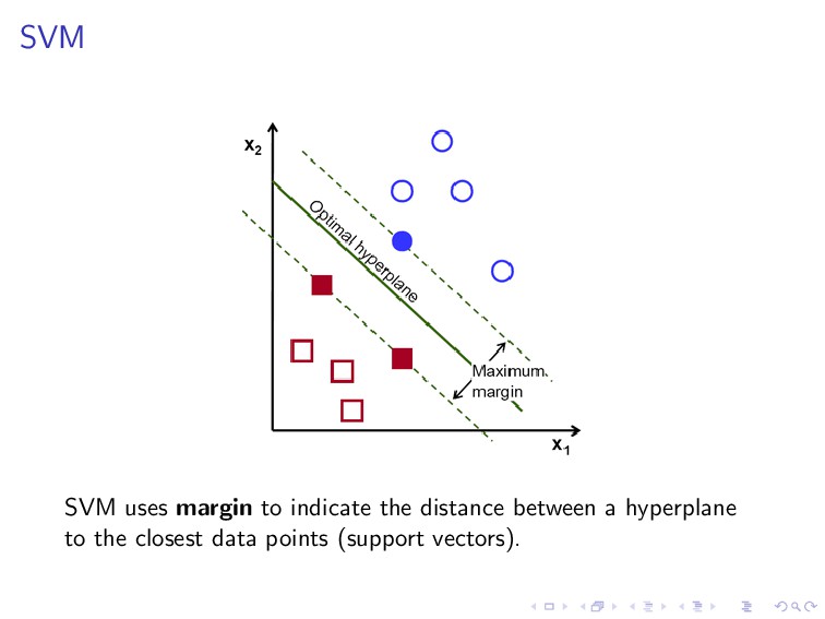
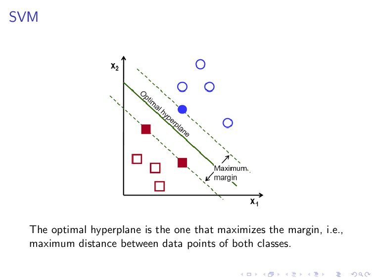
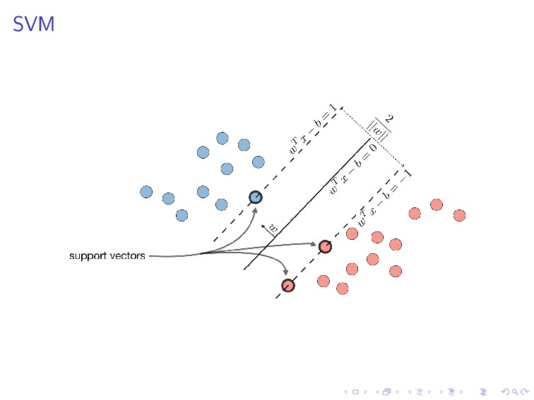
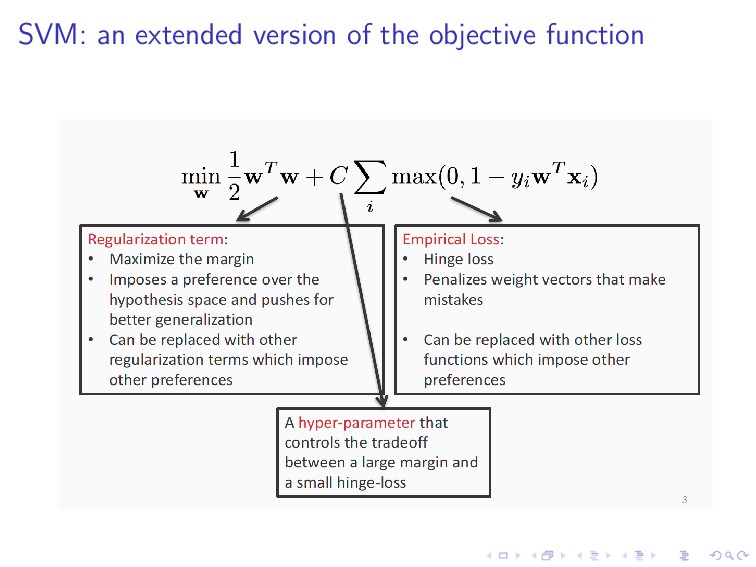
(w, b) are the solution of the following constrained optimization problem. minimize 1 2 ||w||2 subject to y(i)(wT x(i) + b) ≥ 1, i = 1, . . . , n. This is the learning procedure of SVM, which is basically in the same spirit of the learning procedure we have described previously, except that here we apply a linear constraint.
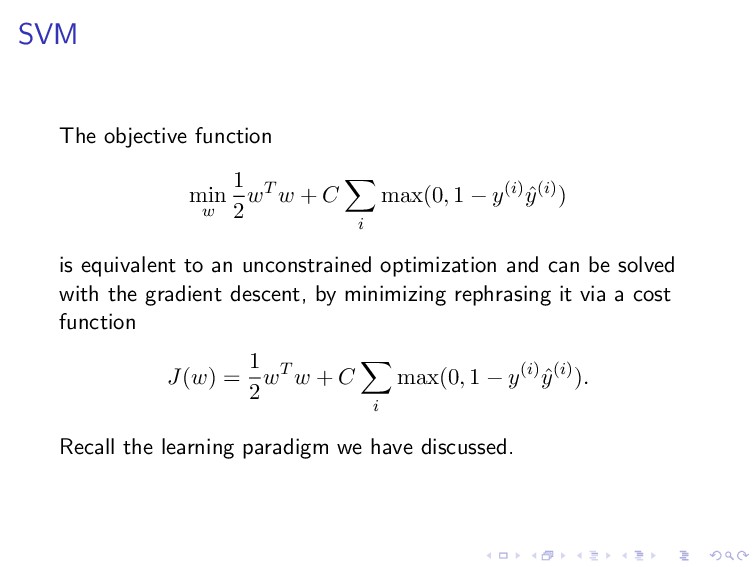
+ C i max(0, 1 − y(i) ˆ y(i)) is equivalent to an unconstrained optimization and can be solved with the gradient descent, by minimizing rephrasing it via a cost function J(w) = 1 2 wT w + C i max(0, 1 − y(i) ˆ y(i)). Recall the learning paradigm we have discussed.
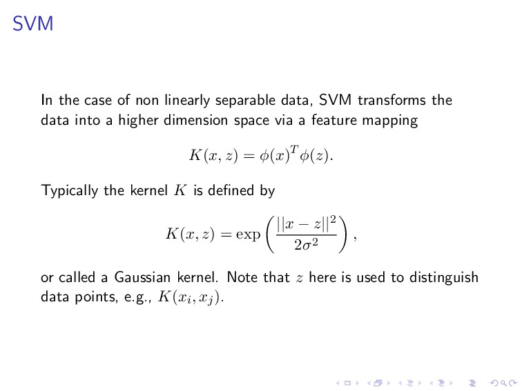
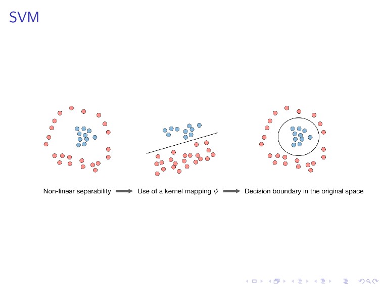
transforms the data into a higher dimension space via a feature mapping K(x, z) = φ(x)T φ(z). Typically the kernel K is defined by K(x, z) = exp ||x − z||2 2σ2 , or called a Gaussian kernel. Note that z here is used to distinguish data points, e.g., K(xi, xj).
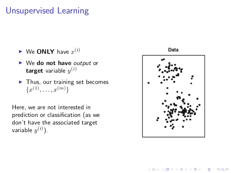
output or target variable y(i) Thus, our training set becomes {x(1), . . . , x(m)} Here, we are not interested in prediction or classification (as we don’t have the associated target variable y(i)).
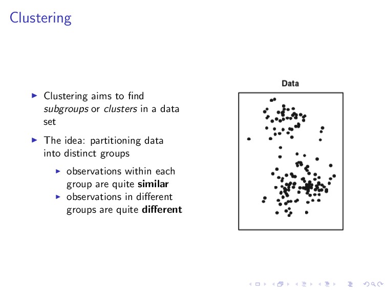
data set The idea: partitioning data into distinct groups observations within each group are quite similar observations in different groups are quite different
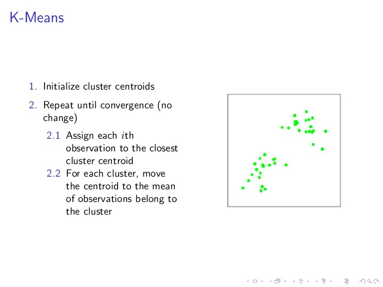
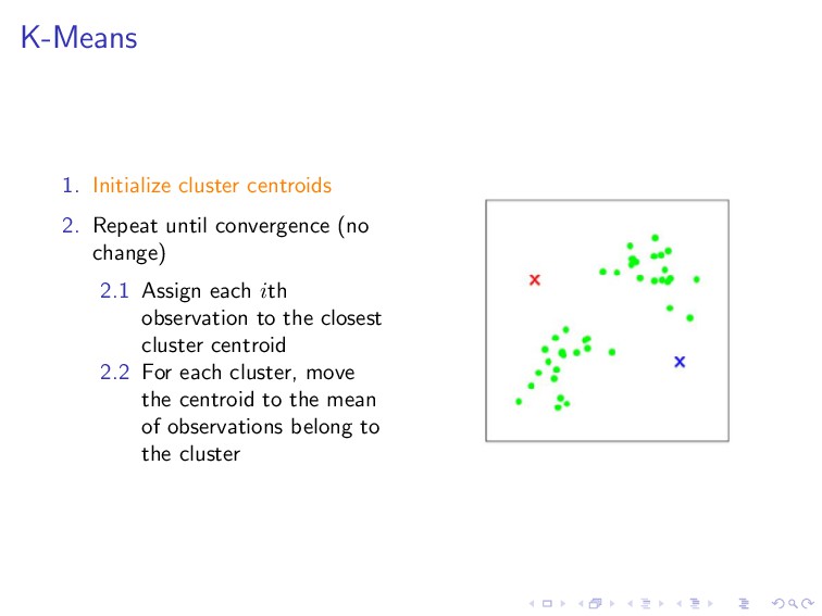
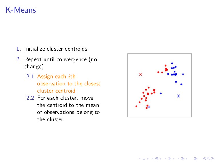
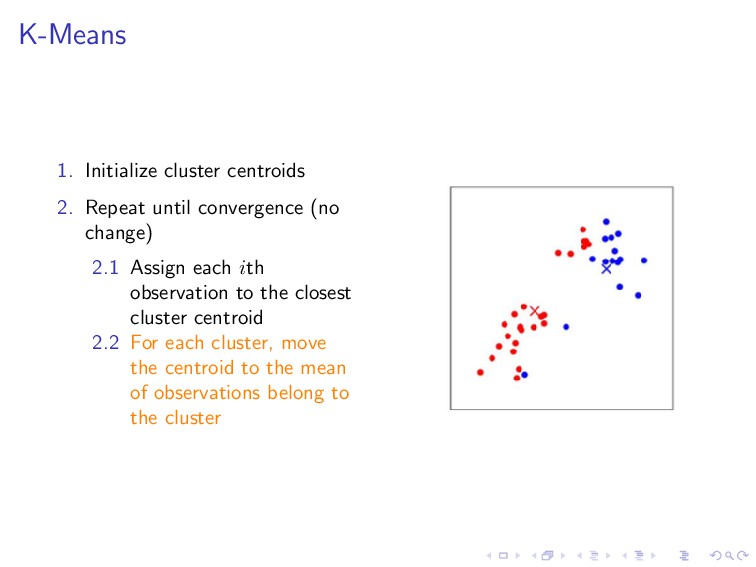
change) 2.1 Assign each ith observation to the closest cluster centroid 2.2 For each cluster, move the centroid to the mean of observations belong to the cluster
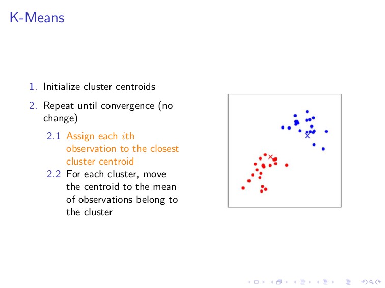
change) 2.1 Assign each ith observation to the closest cluster centroid 2.2 For each cluster, move the centroid to the mean of observations belong to the cluster
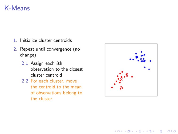
change) 2.1 Assign each ith observation to the closest cluster centroid 2.2 For each cluster, move the centroid to the mean of observations belong to the cluster
change) 2.1 Assign each ith observation to the closest cluster centroid 2.2 For each cluster, move the centroid to the mean of observations belong to the cluster
change) 2.1 Assign each ith observation to the closest cluster centroid 2.2 For each cluster, move the centroid to the mean of observations belong to the cluster
change) 2.1 Assign each ith observation to the closest cluster centroid 2.2 For each cluster, move the centroid to the mean of observations belong to the cluster
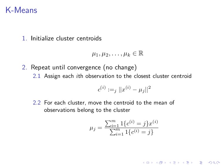
, µk ∈ R 2. Repeat until convergence (no change) 2.1 Assign each ith observation to the closest cluster centroid c(i) :=j ||x(i) − µj ||2 2.2 For each cluster, move the centroid to the mean of observations belong to the cluster µj = m i=1 1{c(i) = j}x(i) m i=1 1{c(i) = j}