Lean Machine Learning

Pycon France 2014

Transcript

1. Lean data science or how to do machine learning with what you have to hand PyconFR – October 26, 2014 – Lyon, France Christophe Bourguignat – AXA Data Innovation Lab - @chris_bour
2. ML Reminder (ML = Machine Learning) ?
3. X = Data ML Reminder (ML = Machine Learning)
4. X = Data y = Answers ML Reminder (ML = Machine Learning)
5. X = Data Train y = Answers ML Reminder (ML = Machine Learning)
6. X = Data Train Unseen Data y = Answers ML Reminder (ML = Machine Learning)
7. ? X = Data Train Unseen Data Prediction y = Answers ML Reminder (ML = Machine Learning)
8. Radiography Of a Typical ML process
9. load Radiography Of a Typical ML process in = read_csv(file)
10. load prepare Radiography Of a Typical ML process in = read_csv(file) f1 = build_feats1(in) … fN = build_featsN(in)
11. load prepare merge Radiography Of a Typical ML process in = read_csv(file) f1 = build_feats1(in) … fN = build_featsN(in) X, y = merge(in, f1, … fN)
12. load prepare merge train Radiography Of a Typical ML process in = read_csv(file) f1 = build_feats1(in) … fN = build_featsN(in) X, y = merge(in, f1, … fN) m = model(params) m.fit(X_train, y_train)
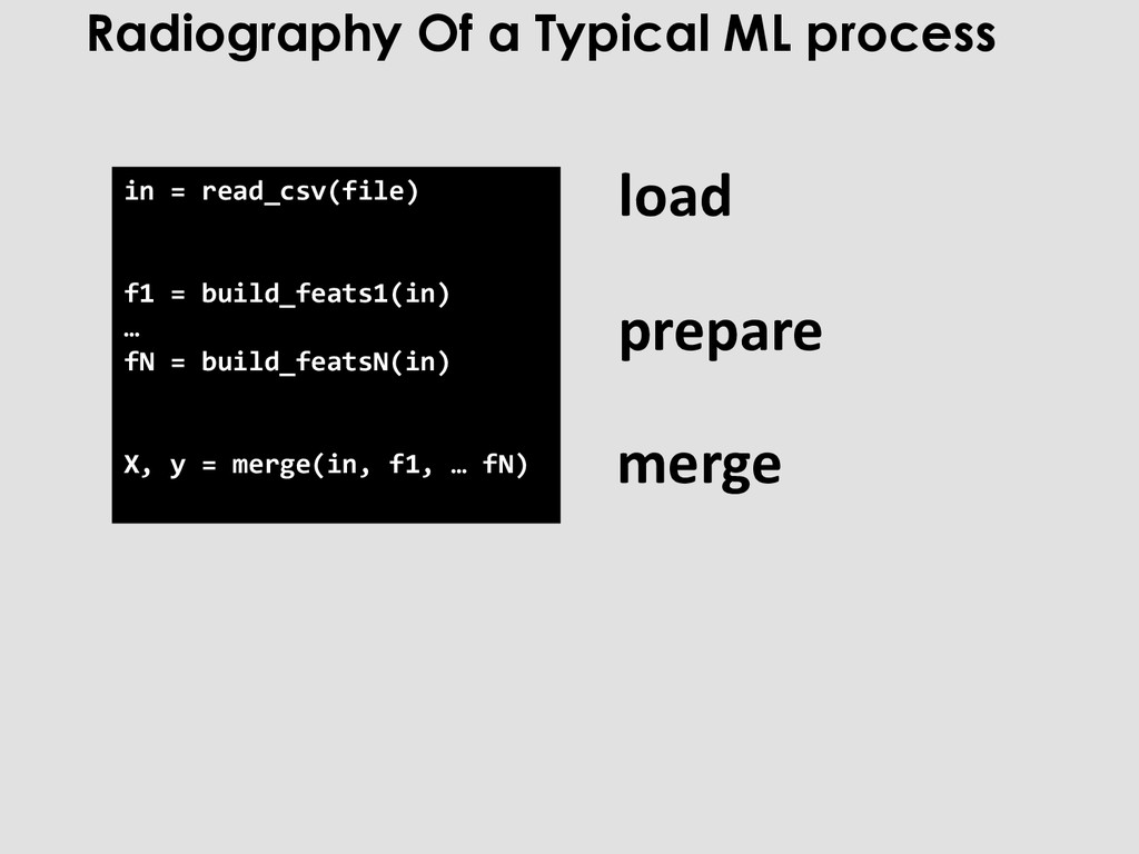
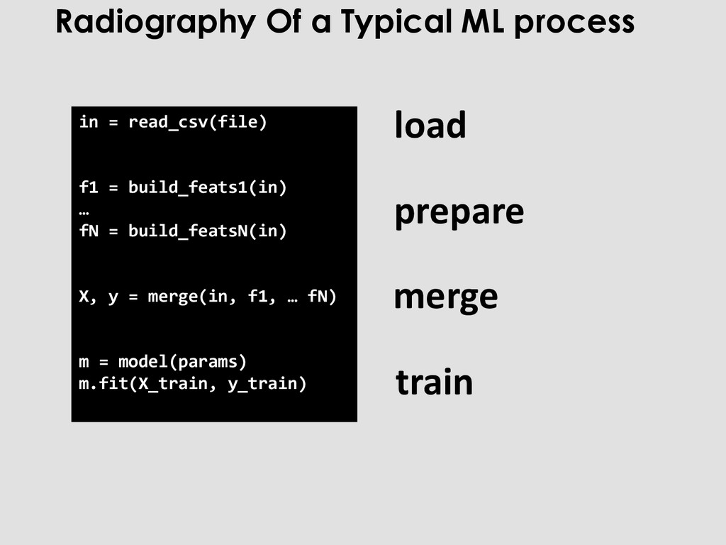
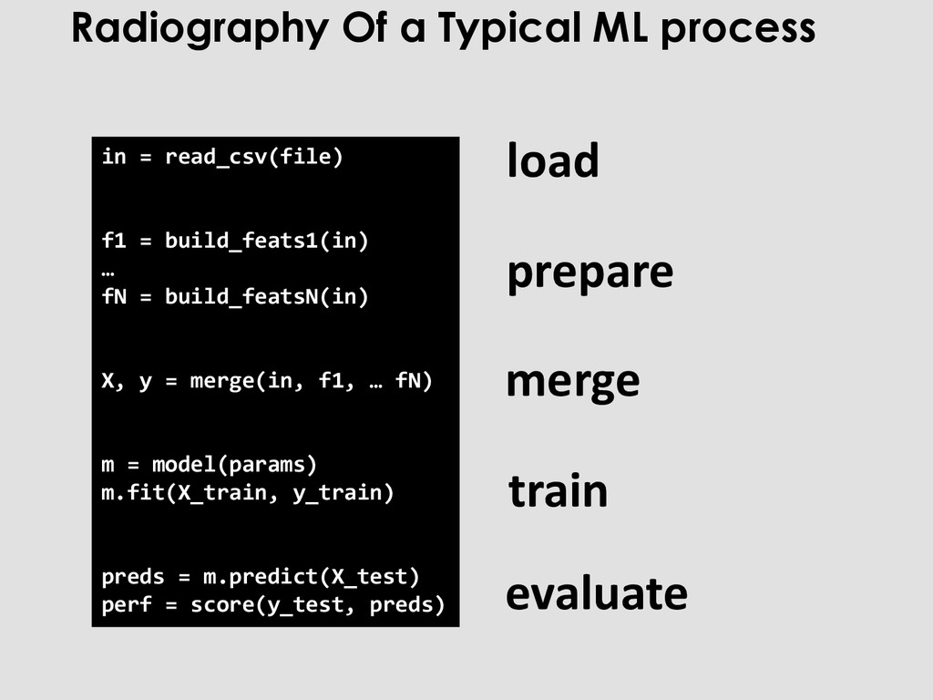
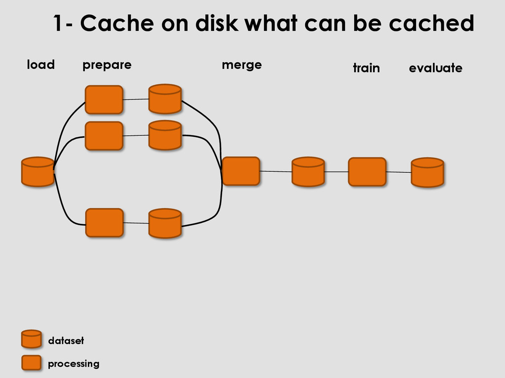
13. in = read_csv(file) f1 = build_feats1(in) … fN = build_featsN(in) X, y = merge(in, f1, … fN) m = model(params) m.fit(X_train, y_train) preds = m.predict(X_test) perf = score(y_test, preds) load prepare merge train evaluate Radiography Of a Typical ML process
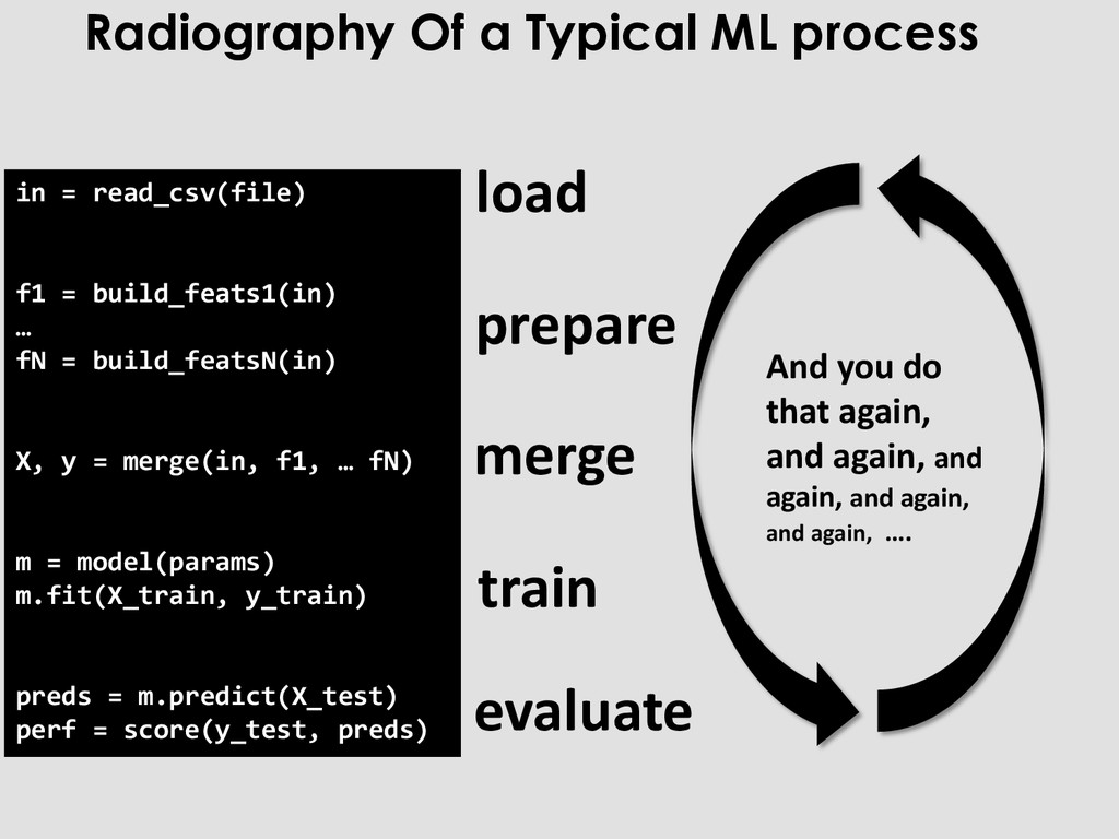
14. in = read_csv(file) f1 = build_feats1(in) … fN = build_featsN(in) X, y = merge(in, f1, … fN) m = model(params) m.fit(X_train, y_train) preds = m.predict(X_test) perf = score(y_test, preds) load prepare merge train evaluate And you do that again, and again, and again, and again, and again, …. Radiography Of a Typical ML process
15. Industry VS personal means
16. Industry VS personal means
17. Let’s try to do lean data science ! or how to do machine learning with what you have to hand
18. Our pythonic weapons Numpy / Scipy Arrays, matrix, linear algebra Pandas Data structures and data analysis Scikit-learn Machine Learning (without learning the Machinery)
19. Numpy / Scipy* Arrays, matrix, linear algebra Pandas* Data structures and data analysis Scikit-learn* Machine Learning (without learning the Machinery) * Coherent ecosystem Our pythonic weapons
20. merge train prepare load evaluate dataset processing 1- Cache on disk what can be cached
21. merge train prepare Don’t run this at each iteration Run only this , by caching Cache this ! load evaluate 1- Cache on disk what can be cached
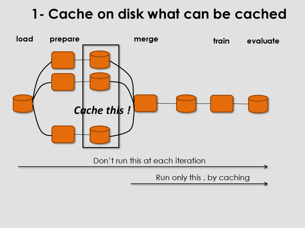
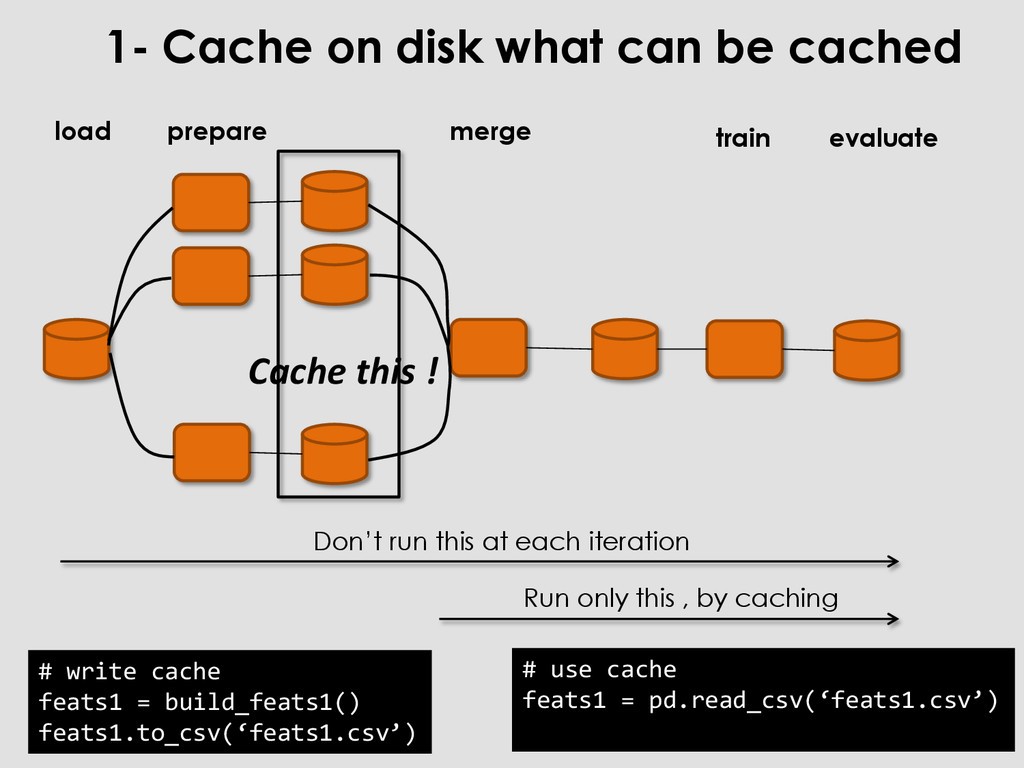
22. # write cache feats1 = build_feats1() feats1.to_csv(‘feats1.csv’) # use cache feats1 = pd.read_csv(‘feats1.csv’) 1- Cache on disk what can be cached merge train prepare Don’t run this at each iteration Run only this , by caching Cache this ! load evaluate
23. 2 - Use sparse matrix representation (when possible) 0 0 0 . . 1 0 0 1 . . 0 0 1 0 . . 0 M =
24. 2 - Use sparse matrix representation (when possible) 0 0 0 . . 1 0 0 1 . . 0 0 1 0 . . 0 from scipy import sparse M = sparse.coo_matrix(M) (2,2) -> 1 (3,7) -> 1 (673,1)-> 1 M = 0 0 0 . . 1 0 0 1 . . 0 0 1 0 . . 0 M =
25. 3 - Use less data (when possible) from sklearn.learning_curve import learning_curve train_sizes, train_scores, test_scores = learning_curve(model, X, y) source : http://alexanderfabisch.github.io/blog/2014/01/12/learning_curves.html
26. 4 - Do online (incremental) learning (when possible) import pandas as pd from sklearn import linear_model model = linear_model.SGDClassifier() train = pd.read_csv(‘train.csv’) model.fit(X, y) X y
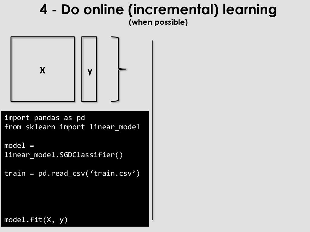
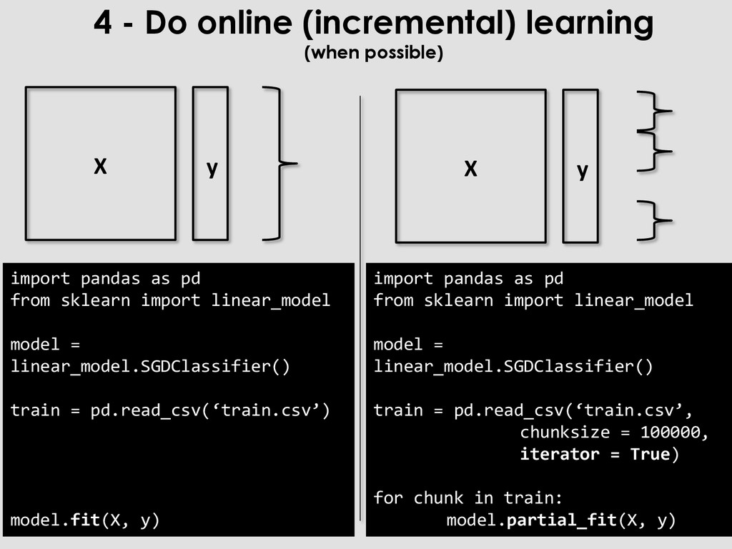
27. 4 - Do online (incremental) learning (when possible) import pandas as pd from sklearn import linear_model model = linear_model.SGDClassifier() train = pd.read_csv(‘train.csv’, chunksize = 100000, iterator = True) for chunk in train: model.partial_fit(X, y) import pandas as pd from sklearn import linear_model model = linear_model.SGDClassifier() train = pd.read_csv(‘train.csv’) model.fit(X, y) X y X y
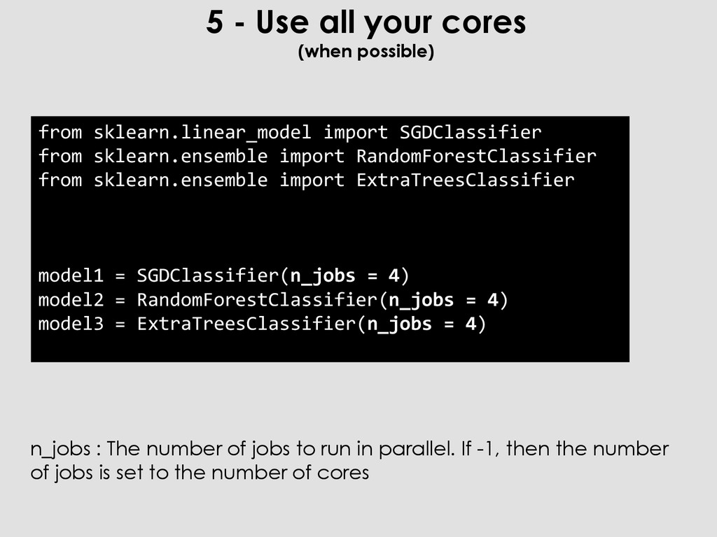
28. 5 - Use all your cores (when possible) from sklearn.linear_model import SGDClassifier from sklearn.ensemble import RandomForestClassifier from sklearn.ensemble import ExtraTreesClassifier model1 = SGDClassifier(n_jobs = 4) model2 = RandomForestClassifier(n_jobs = 4) model3 = ExtraTreesClassifier(n_jobs = 4) n_jobs : The number of jobs to run in parallel. If -1, then the number of jobs is set to the number of cores
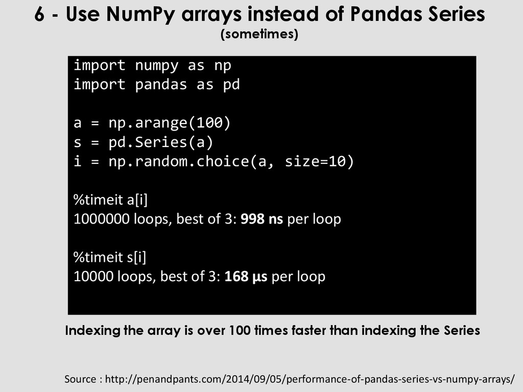
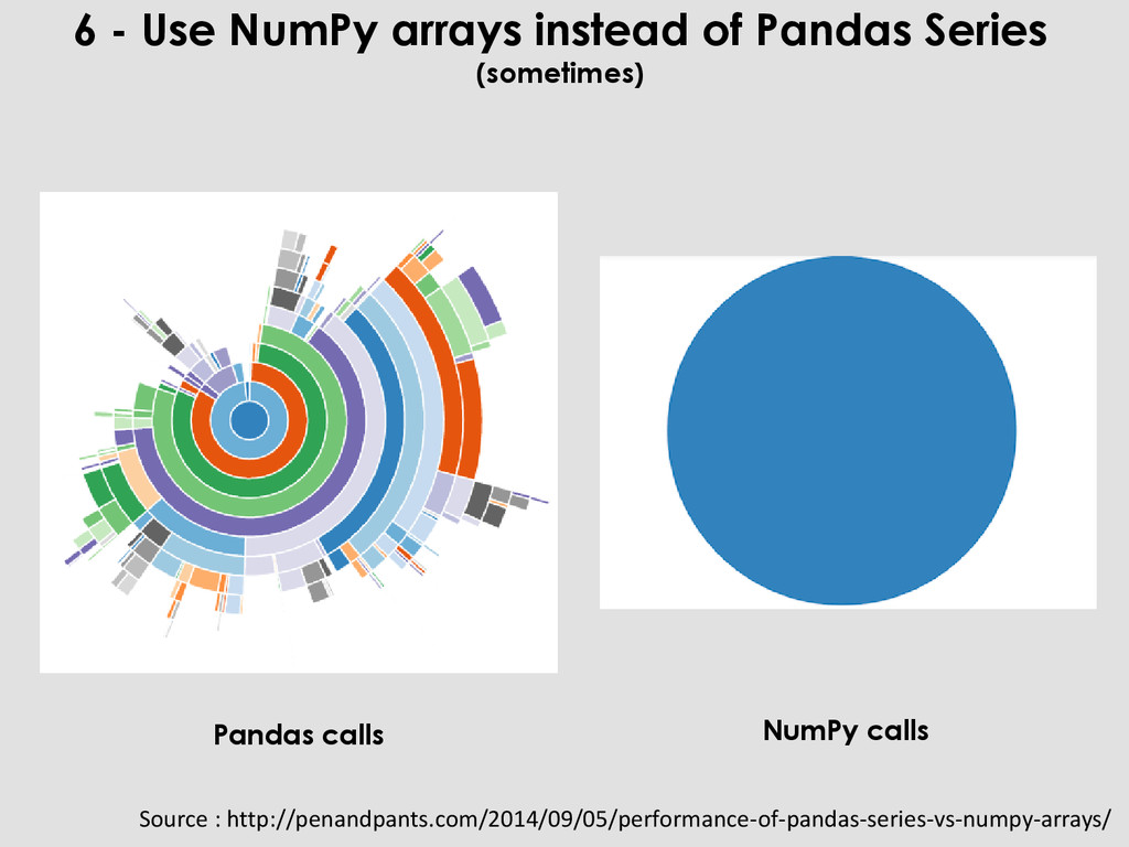
29. import numpy as np import pandas as pd a = np.arange(100) s = pd.Series(a) i = np.random.choice(a, size=10) %timeit a[i] 1000000 loops, best of 3: 998 ns per loop %timeit s[i] 10000 loops, best of 3: 168 µs per loop 6 - Use NumPy arrays instead of Pandas Series (sometimes) Source : http://penandpants.com/2014/09/05/performance-of-pandas-series-vs-numpy-arrays/ Indexing the array is over 100 times faster than indexing the Series
30. Source : http://penandpants.com/2014/09/05/performance-of-pandas-series-vs-numpy-arrays/ Pandas calls NumPy calls 6 - Use NumPy arrays instead of Pandas Series (sometimes)
31. And also … - PyPy, Numba, Cython - Accelerating Python (as quickly as a compiled languages) with just in time compilation - Advanced NumPy optimization techniques - strides : tuple of bytes to step in each dimension when traversing an array - memmap : Memory-mapped files accessing small segments of large files on disk, without reading the entire file into memory
32. Thank you – Questions ?
33. BONUS
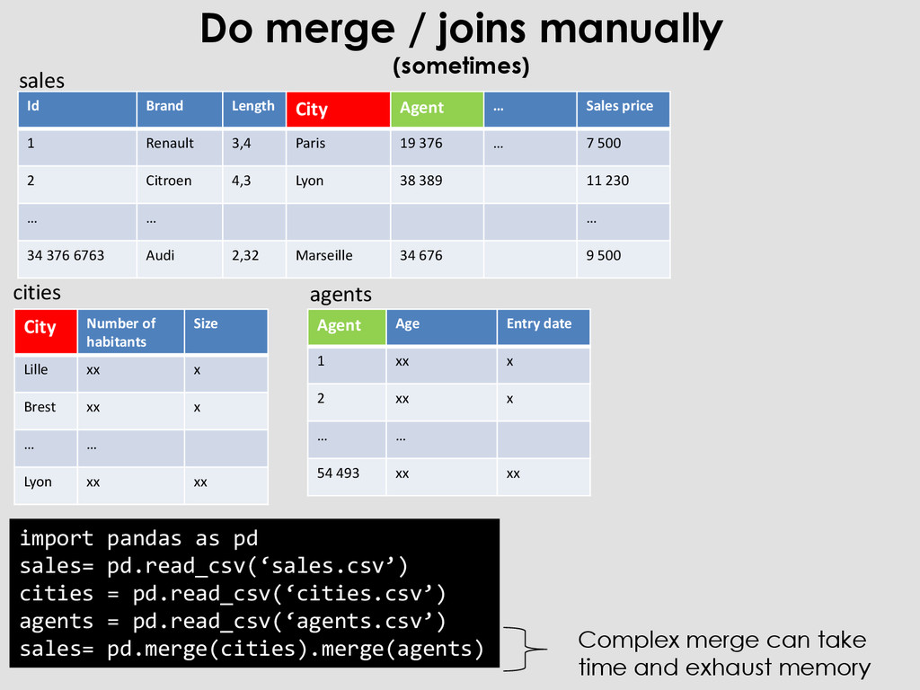
34. Do merge / joins manually (sometimes) Id Brand Length City Agent … Sales price 1 Renault 3,4 Paris 19 376 … 7 500 2 Citroen 4,3 Lyon 38 389 11 230 … … … 34 376 6763 Audi 2,32 Marseille 34 676 9 500 City Number of habitants Size Lille xx x Brest xx x … … Lyon xx xx Agent Age Entry date 1 xx x 2 xx x … … 54 493 xx xx import pandas as pd sales= pd.read_csv(‘sales.csv’) cities = pd.read_csv(‘cities.csv’) agents = pd.read_csv(‘agents.csv’) sales= pd.merge(cities).merge(agents) sales cities agents Complex merge can take time and exhaust memory
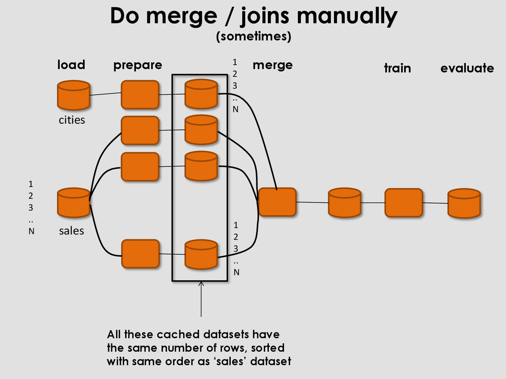
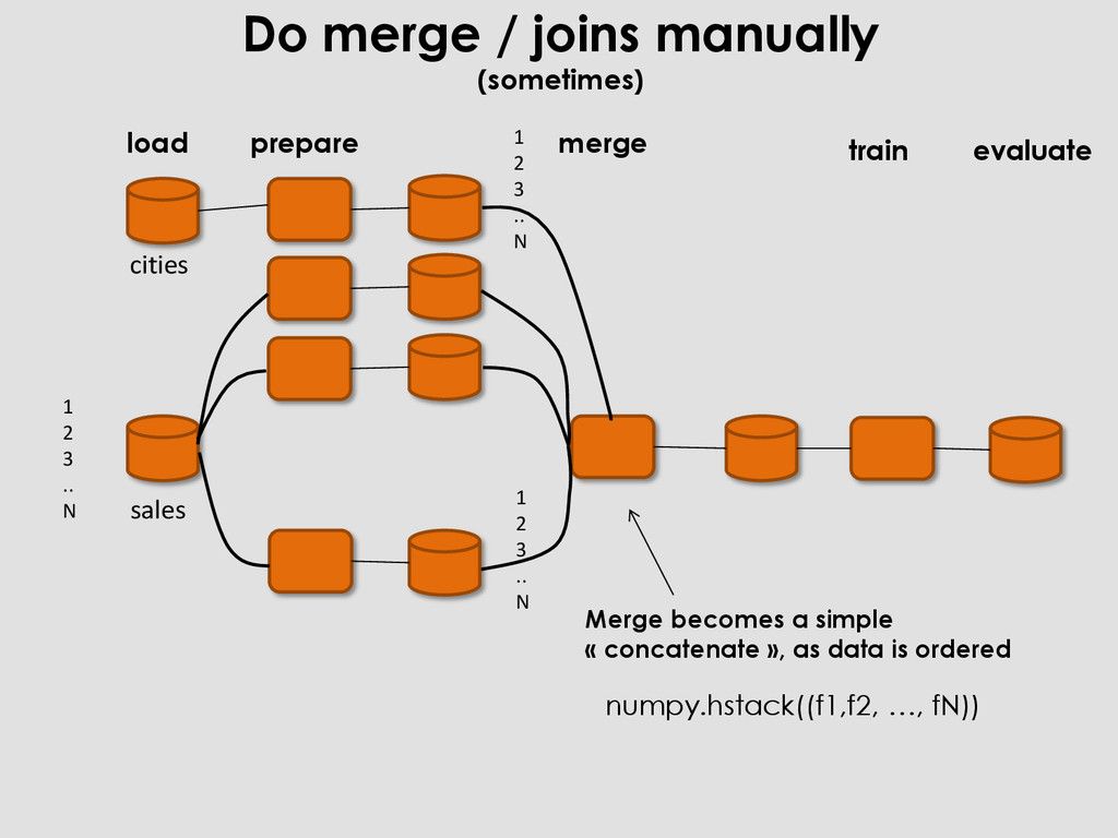
35. Do merge / joins manually (sometimes) sales cities merge train prepare load evaluate 1 2 3 .. N 1 2 3 .. N 1 2 3 .. N All these cached datasets have the same number of rows, sorted with same order as ‘sales’ dataset
36. Do merge / joins manually (sometimes) sales cities merge train prepare load evaluate 1 2 3 .. N 1 2 3 .. N 1 2 3 .. N Merge becomes a simple « concatenate », as data is ordered numpy.hstack((f1,f2, …, fN))
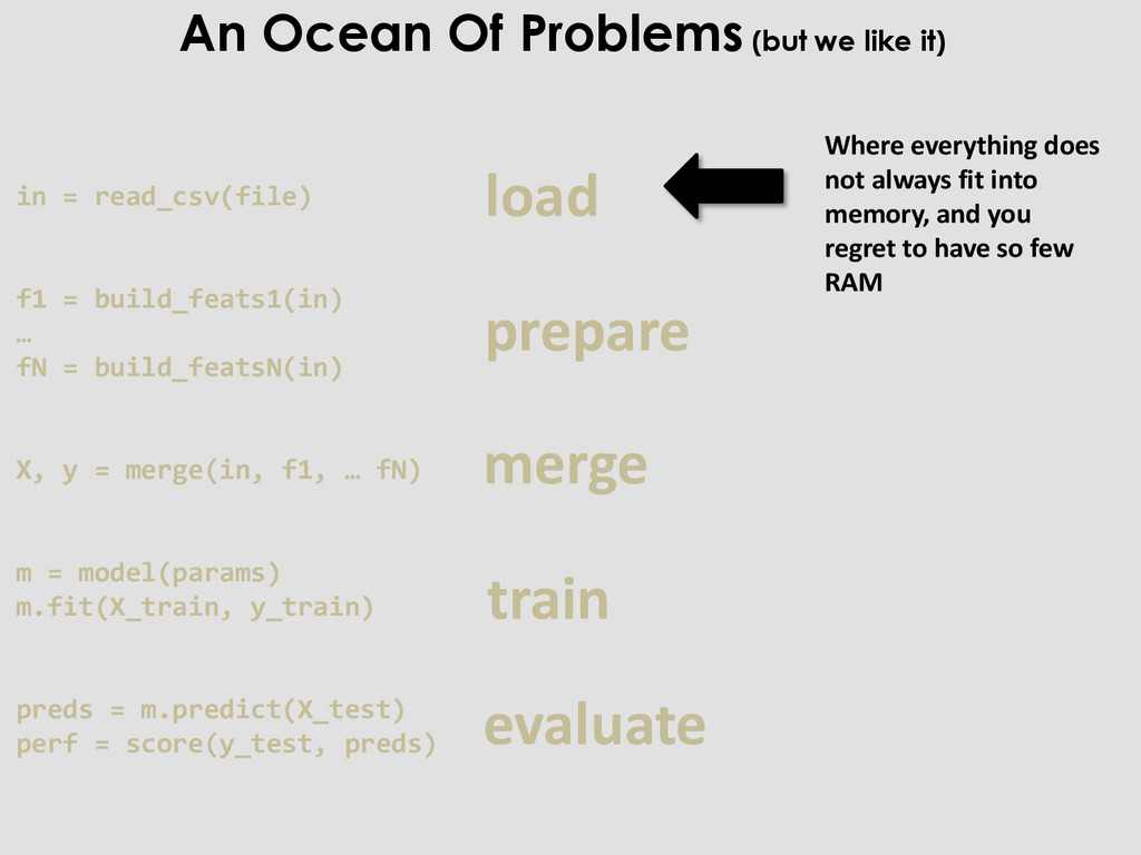
37. An Ocean Of Problems (but we like it) load prepare merge train evaluate Where everything does not always fit into memory, and you regret to have so few RAM in = read_csv(file) f1 = build_feats1(in) … fN = build_featsN(in) X, y = merge(in, f1, … fN) m = model(params) m.fit(X_train, y_train) preds = m.predict(X_test) perf = score(y_test, preds)
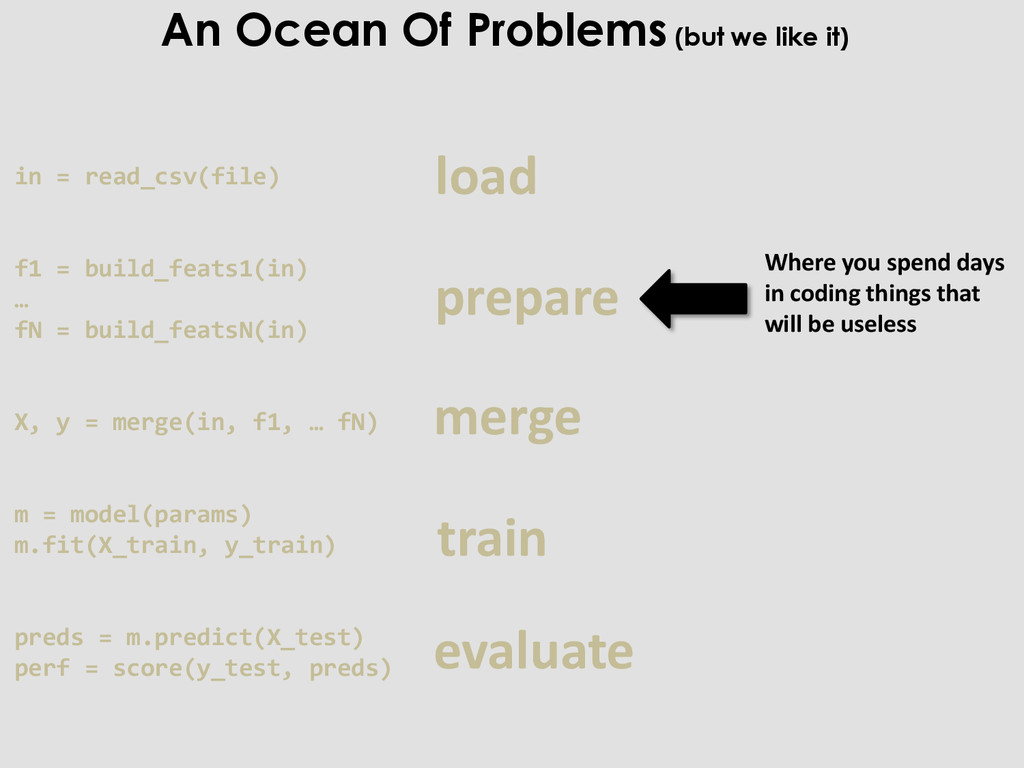
38. load prepare merge train evaluate Where you spend days in coding things that will be useless in = read_csv(file) f1 = build_feats1(in) … fN = build_featsN(in) X, y = merge(in, f1, … fN) m = model(params) m.fit(X_train, y_train) preds = m.predict(X_test) perf = score(y_test, preds) An Ocean Of Problems (but we like it)
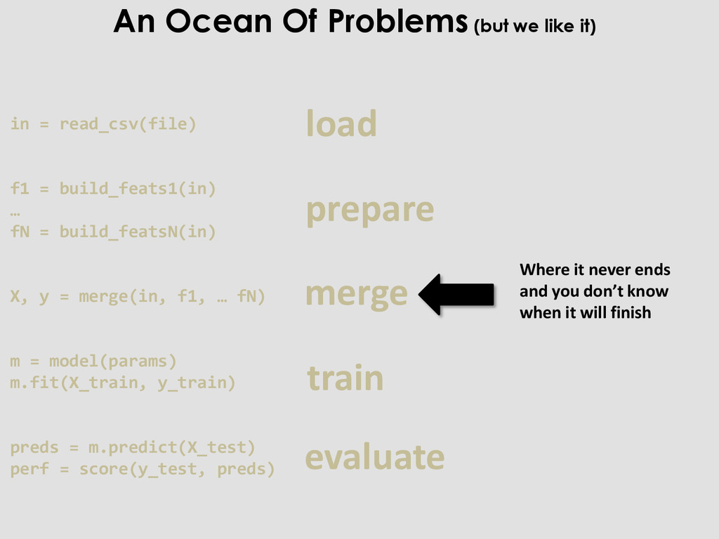
39. load prepare merge train evaluate Where it never ends and you don’t know when it will finish in = read_csv(file) f1 = build_feats1(in) … fN = build_featsN(in) X, y = merge(in, f1, … fN) m = model(params) m.fit(X_train, y_train) preds = m.predict(X_test) perf = score(y_test, preds) An Ocean Of Problems (but we like it)
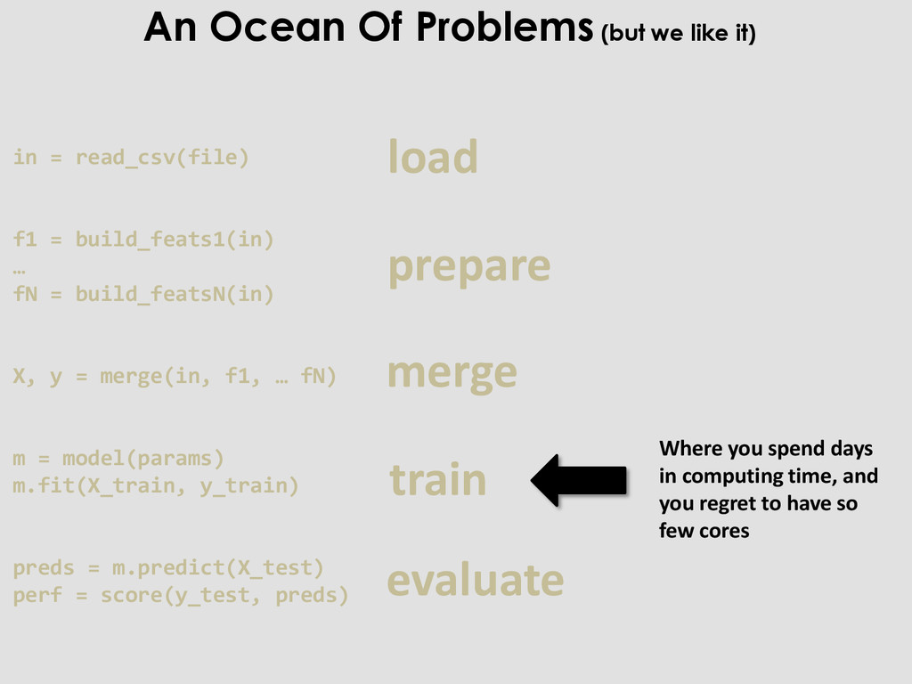
40. load prepare merge train evaluate Where you spend days in computing time, and you regret to have so few cores in = read_csv(file) f1 = build_feats1(in) … fN = build_featsN(in) X, y = merge(in, f1, … fN) m = model(params) m.fit(X_train, y_train) preds = m.predict(X_test) perf = score(y_test, preds) An Ocean Of Problems (but we like it)
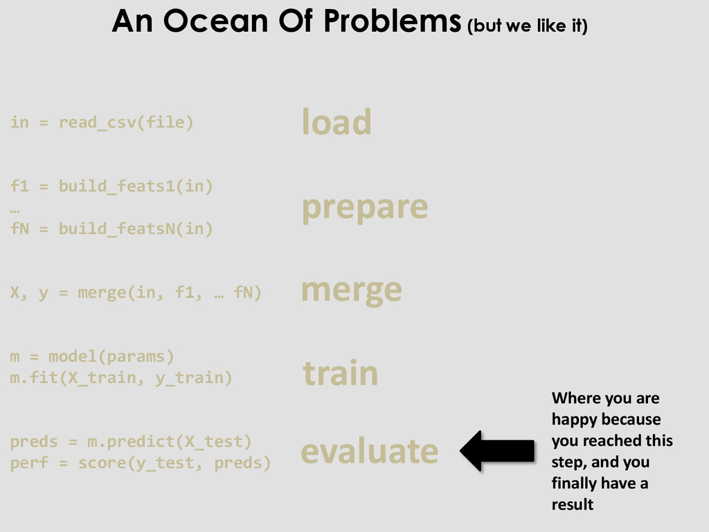
41. load prepare merge train evaluate Where you are happy because you reached this step, and you finally have a result in = read_csv(file) f1 = build_feats1(in) … fN = build_featsN(in) X, y = merge(in, f1, … fN) m = model(params) m.fit(X_train, y_train) preds = m.predict(X_test) perf = score(y_test, preds) An Ocean Of Problems (but we like it)
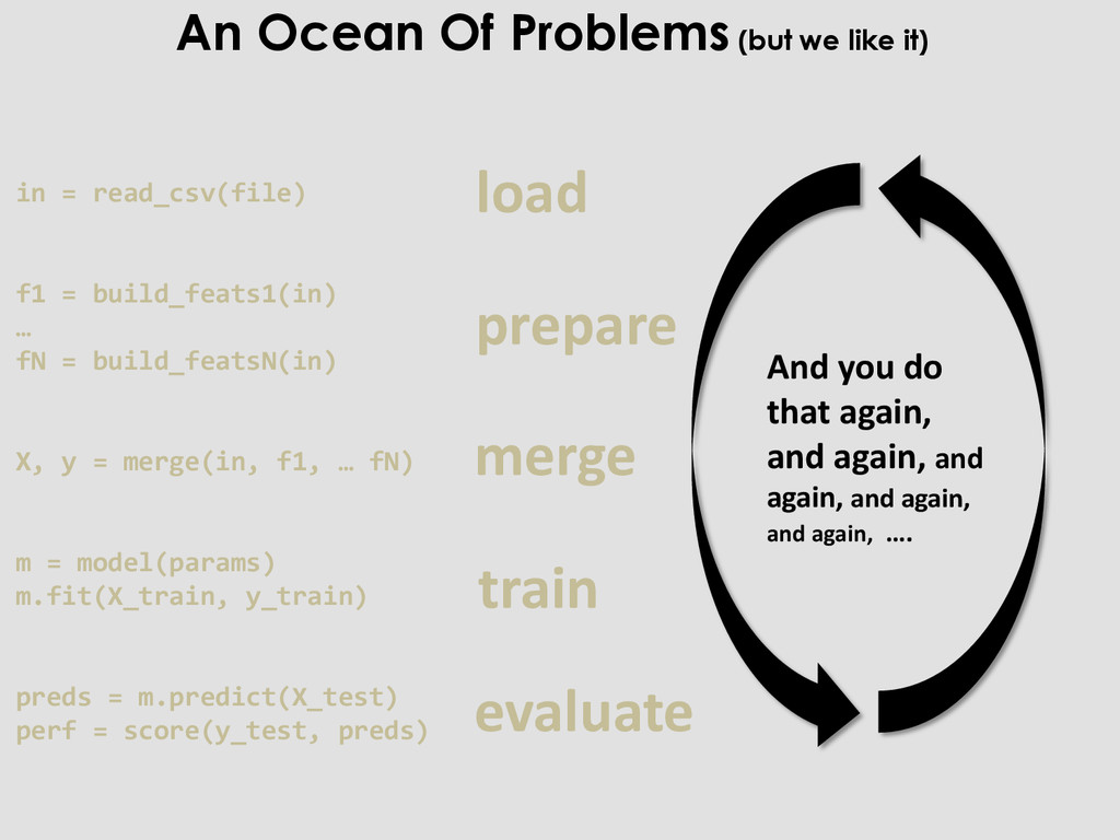
42. in = read_csv(file) f1 = build_feats1(in) … fN = build_featsN(in) X, y = merge(in, f1, … fN) m = model(params) m.fit(X_train, y_train) preds = m.predict(X_test) perf = score(y_test, preds) load prepare merge train evaluate And you do that again, and again, and again, and again, and again, …. An Ocean Of Problems (but we like it)