2025 LIBD lcolladotor data science team TL;DR

A recap of recent work from our R Bioconductor-powered Team Data Science group at the Lieber Institute for Data Science.

Team website: https://lcolladotor.github.io/

Topics Presented & Presenters:
1. Spatially Resolved Transcriptomics with Visium - Manisha Barse
2. Visium HD data analysis - Nick Eagles
3. sc/snRNA-seq data analysis - Melissa Mayén Quiroz
4. Multi-ome data analysis - Cynthia Soto Cardinault
5. Bulk RNA-seq deconvolution - Louise Huuki-Myers
6. Bulk RNA-seq data analysis - Louise Huuki-Myers & Nick Eagles
7. qsvaR - Nick Eagles
8. CHESS-Brain - Geo Pertea
9. Open Source Software Development - Nick Eagles
10. JHPCE - Nick Eagles
11. LIBD rstats & journal clubs - Nick Eages

1. @lcolladotor.bsky.social lcolladotor.github.io lcolladotor.github.io/bioc_team_ds R Bioconductor-powered Team Data Science Data Science Team 1, Translational Neuroscience Division Leonardo Collado Torres, LIBD Investigator + Asst. Prof. Johns Hopkins Biostatistics January 29th, 2025 Slides available at speakerdeck.com/lcolladotor Orchestrated By Louise Huuki-Myers
2. Spatially Resolved Transcriptomics with Visium Presented By Manisha Barse
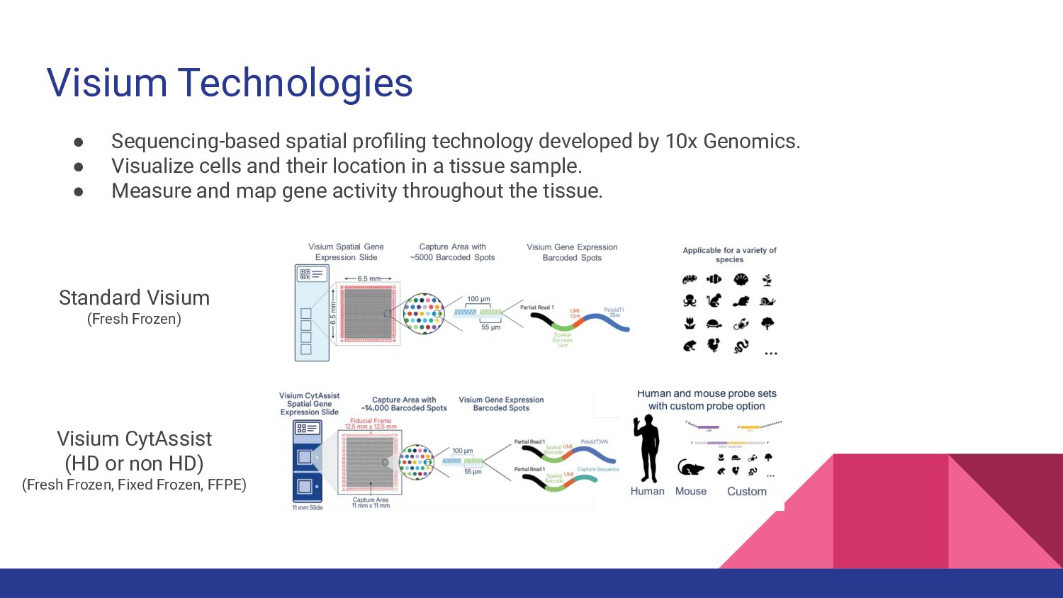
3. Visium Technologies Standard Visium (Fresh Frozen) Visium CytAssist (HD or non HD) (Fresh Frozen, Fixed Frozen, FFPE) • Sequencing-based spatial profiling technology developed by 10x Genomics. • Visualize cells and their location in a tissue sample. • Measure and map gene activity throughout the tissue.
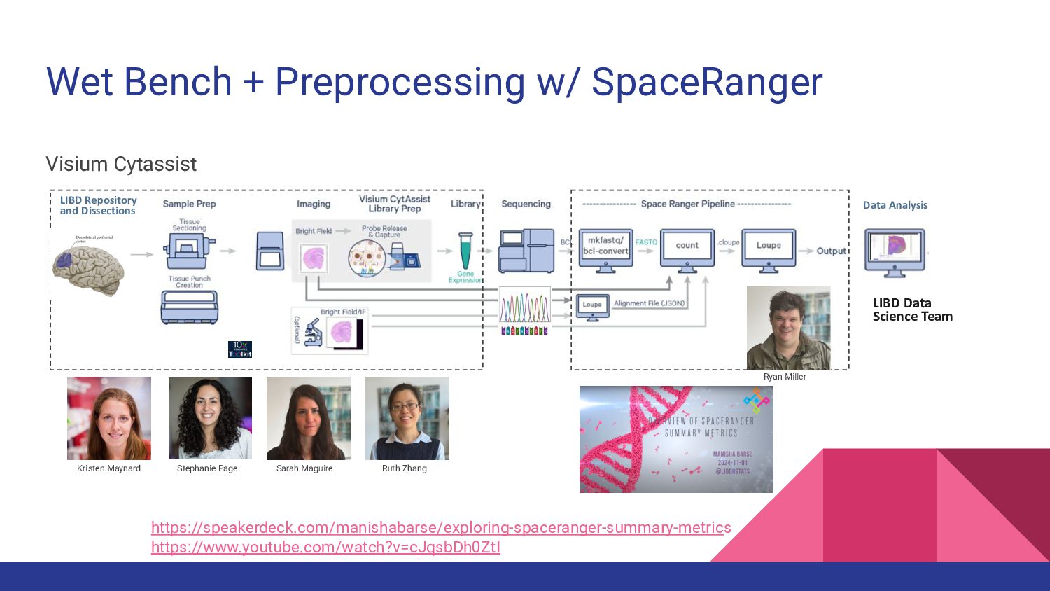
4. Wet Bench + Preprocessing w/ SpaceRanger Visium Cytassist LIBD Repository and Dissections Kristen Maynard Stephanie Page Sarah Maguire Ruth Zhang Ryan Miller Data Analysis https://speakerdeck.com/manishabarse/exploring-spaceranger-summary-metrics https://www.youtube.com/watch?v=cJqsbDh0ZtI LIBD Data Science Team
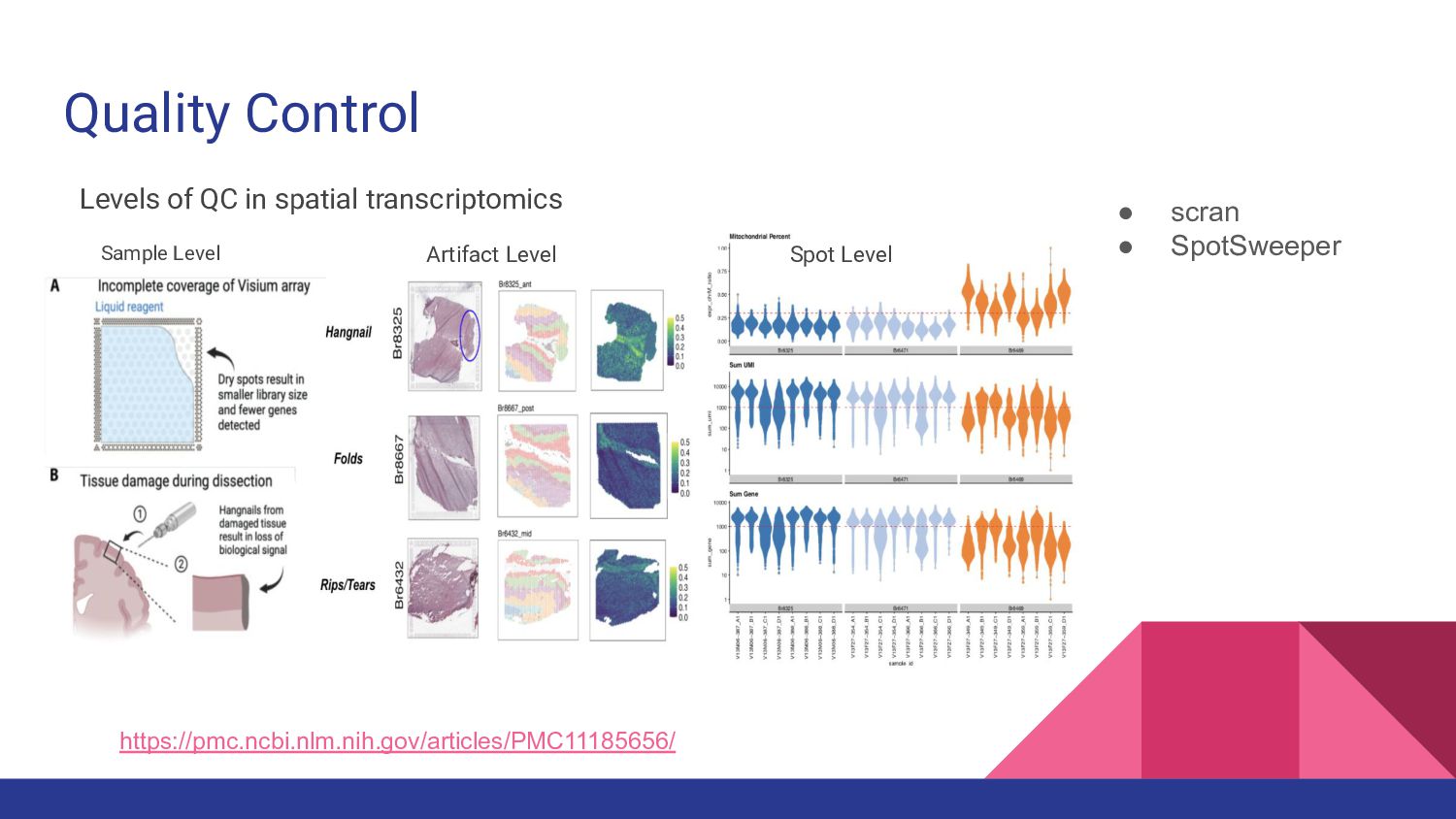
5. Quality Control Levels of QC in spatial transcriptomics Artifact Level Spot Level https://pmc.ncbi.nlm.nih.gov/articles/PMC11185656/ Sample Level • scran • SpotSweeper
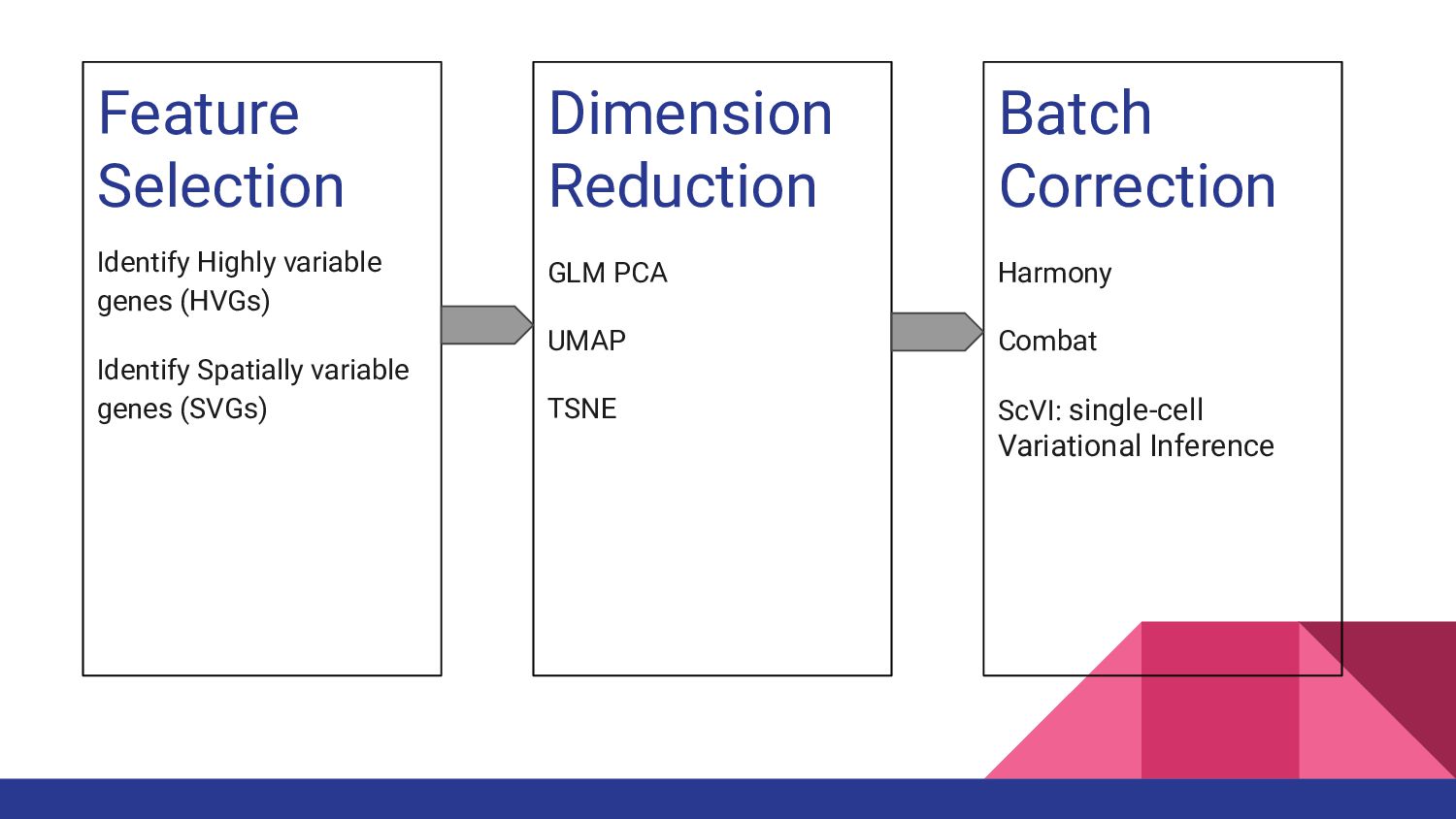
6. Feature Selection Identify Highly variable genes (HVGs) Identify Spatially variable genes (SVGs) Dimension Reduction GLM PCA UMAP TSNE Batch Correction Harmony Combat ScVI: single-cell Variational Inference
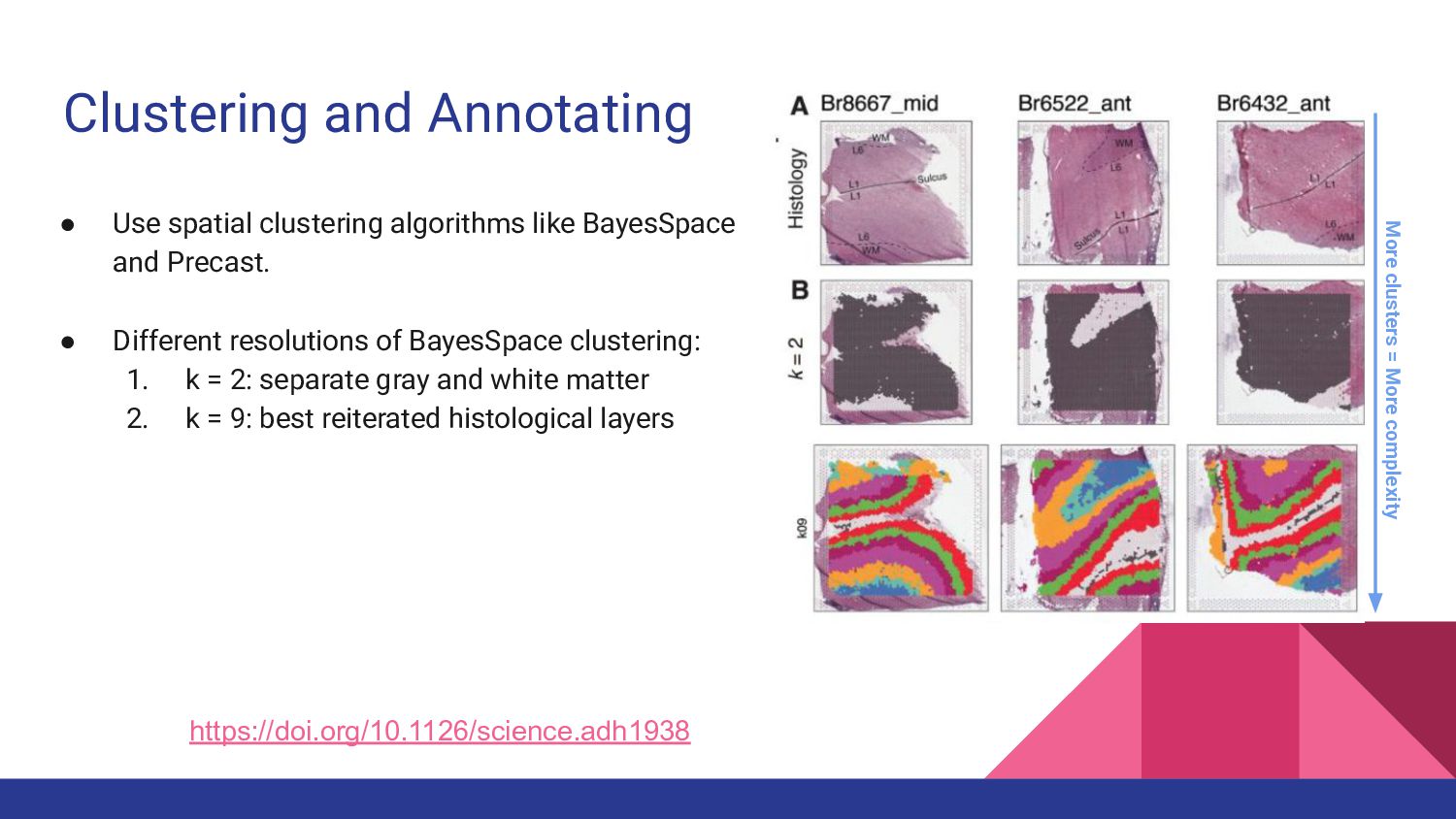
7. Clustering and Annotating • Use spatial clustering algorithms like BayesSpace and Precast. • Different resolutions of BayesSpace clustering: 1. k = 2: separate gray and white matter 2. k = 9: best reiterated histological layers https://doi.org/10.1126/science.adh1938 More clusters = More complexity
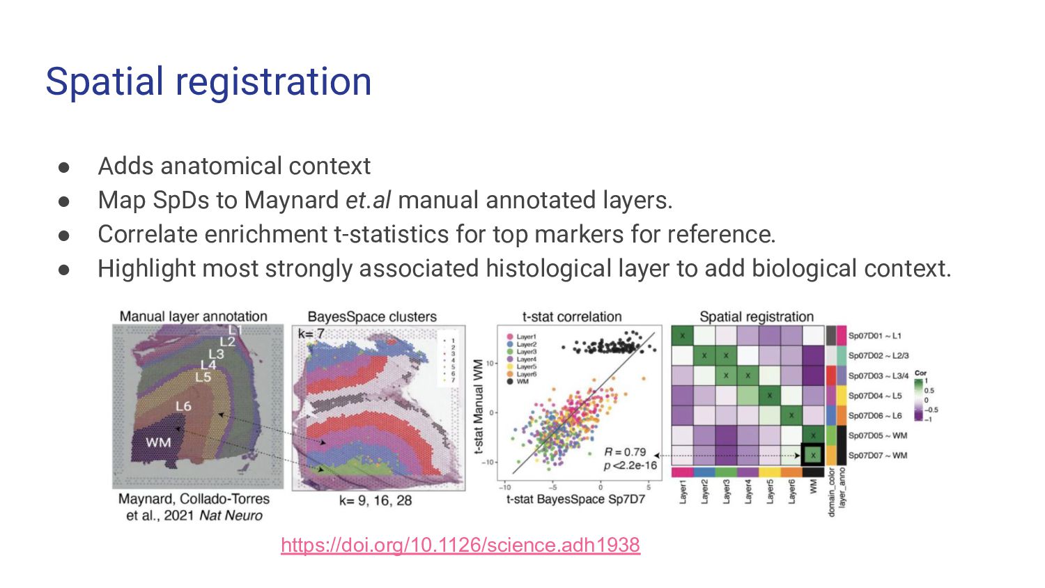
8. Spatial registration • Adds anatomical context • Map SpDs to Maynard et.al manual annotated layers. • Correlate enrichment t-statistics for top markers for reference. • Highlight most strongly associated histological layer to add biological context. https://doi.org/10.1126/science.adh1938
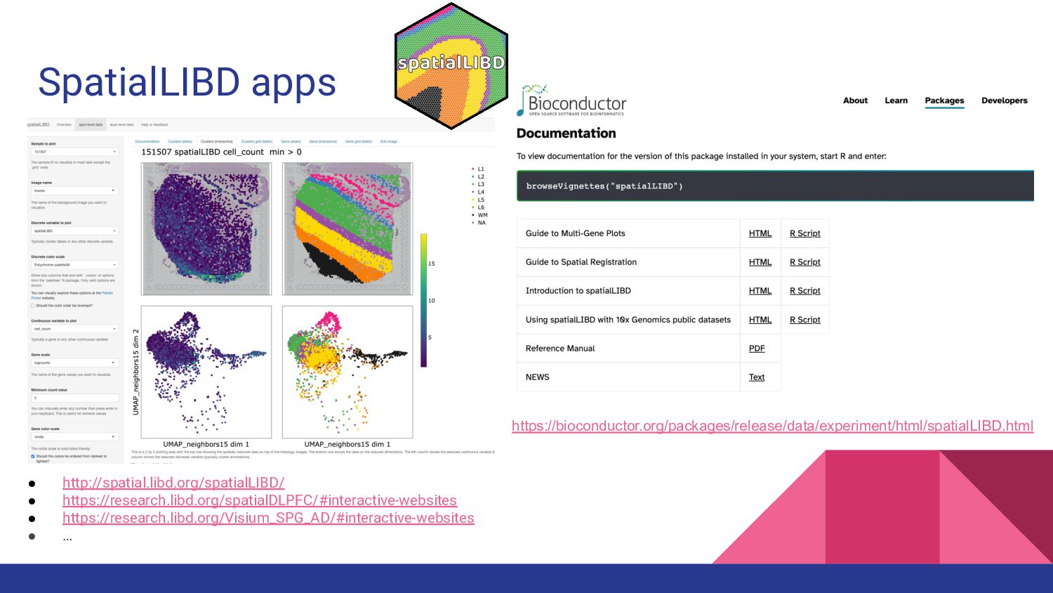
9. SpatialLIBD apps • http://spatial.libd.org/spatialLIBD/ • https://research.libd.org/spatialDLPFC/#interactive-websites • https://research.libd.org/Visium_SPG_AD/#interactive-websites • … https://bioconductor.org/packages/release/data/experiment/html/spatialLIBD.html
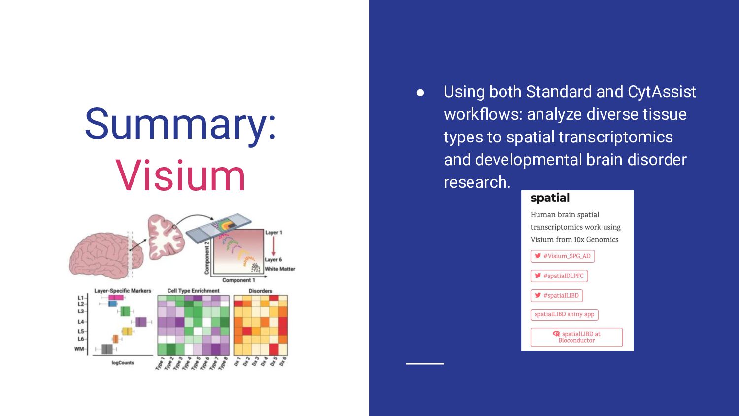
10. Summary: Visium • Using both Standard and CytAssist workflows: analyze diverse tissue types to spatial transcriptomics and developmental brain disorder research.
11. Visium HD data analysis Presented By Nick Eagles
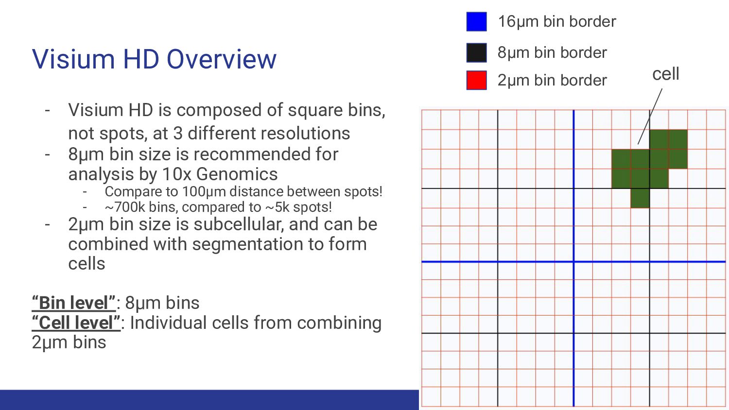
12. Visium HD Overview - Visium HD is composed of square bins, not spots, at 3 different resolutions - 8μm bin size is recommended for analysis by 10x Genomics - Compare to 100μm distance between spots! - ~700k bins, compared to ~5k spots! - 2μm bin size is subcellular, and can be combined with segmentation to form cells “Bin level”: 8μm bins “Cell level”: Individual cells from combining 2μm bins 16μm bin border 8μm bin border 2μm bin border cell
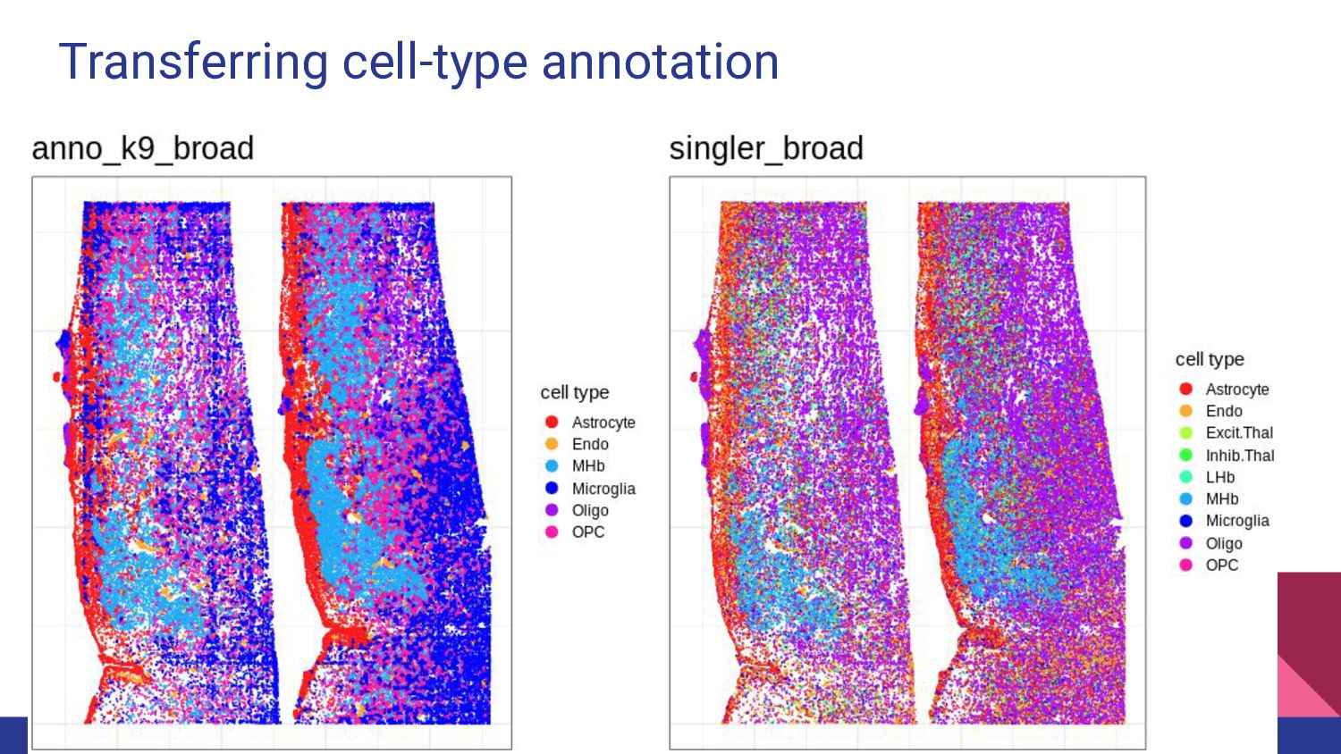
13. Visium HD: Goals and Challenges Goals: - Explore the current landscape of Visium HD software tools - What’s useful and feasible to run on our data? - Develop novel code where there are holes - Gain interesting insights from LIBD Visium HD datasets (e.g. habenula, DLPFC, HPC samples) - What questions can we answer with spatially resolved cells? Challenges: - Big data: 1 HD sample is larger than 100 standard samples - Uncharted territory; limited existing solutions
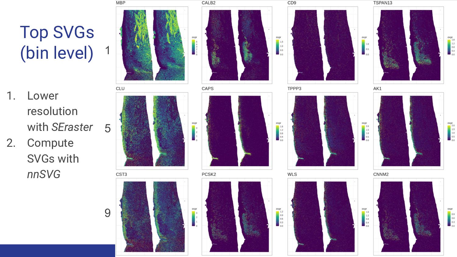
14. Top SVGs (bin level) 1. Lower resolution with SEraster 2. Compute SVGs with nnSVG 1 5 9
15. FICTURE: habenula * Note: mirrored and rotated data
16. Banksy cell-level clusters k = 2 k = 4 k = 9
17. Transferring cell-type annotation
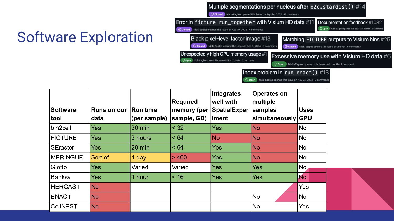
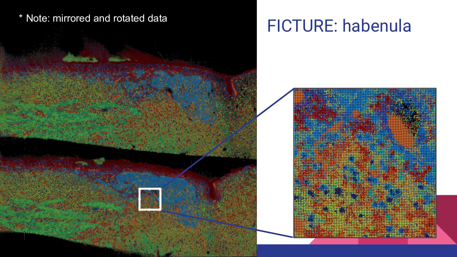
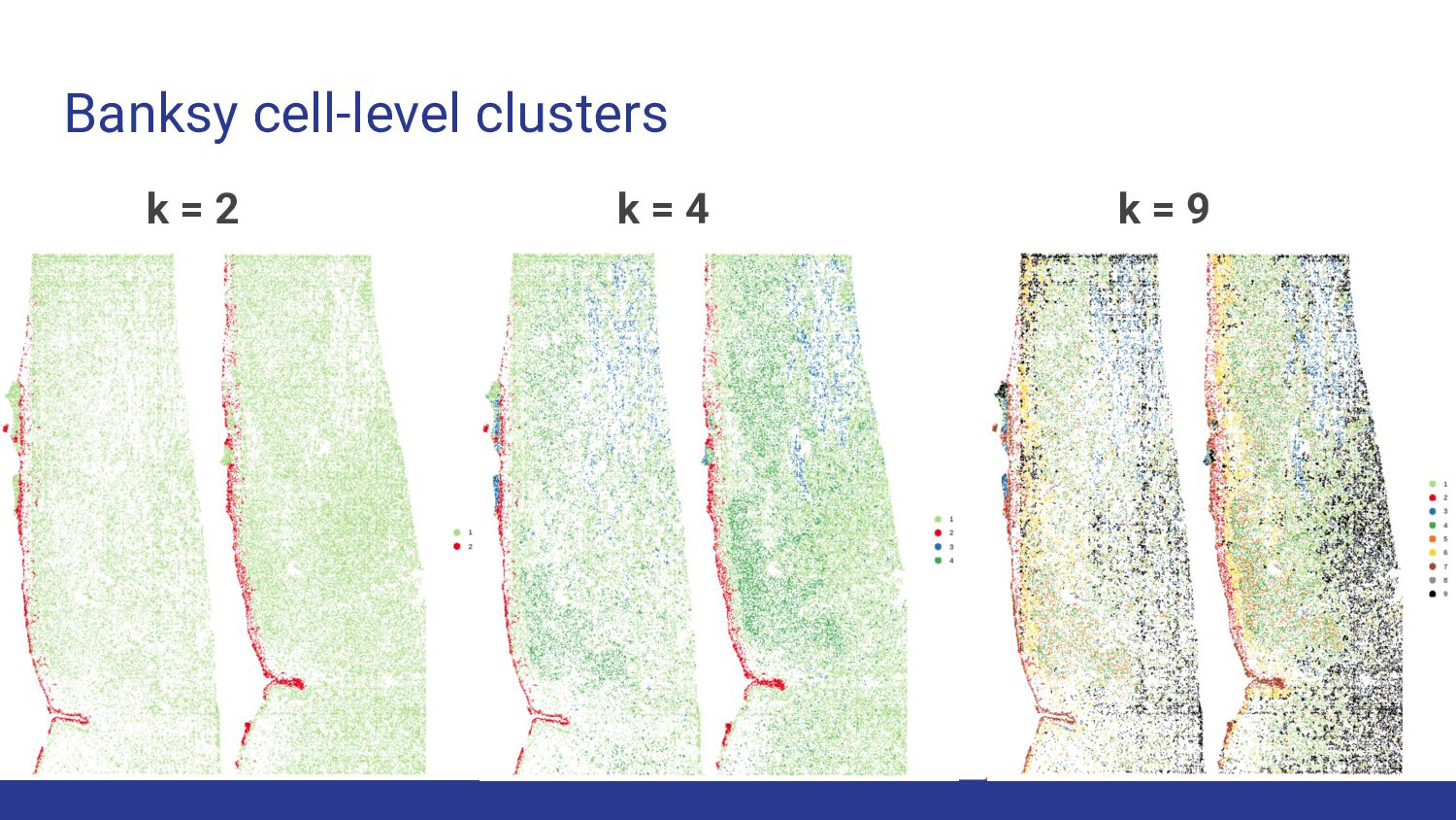
18. Software Exploration Software tool Runs on our data Run time (per sample) Required memory (per sample, GB) Integrates well with SpatialExper iment Operates on multiple samples simultaneously Uses GPU bin2cell Yes 30 min < 32 Yes No No FICTURE Yes 3 hours < 64 No No No SEraster Yes 20 min < 64 Yes No No MERINGUE Sort of 1 day > 400 Yes No No Giotto Yes Varied Varied Yes Yes No Banksy Yes 1 hour < 16 Yes Yes No HERGAST No Yes ENACT No No No CellNEST No No Yes
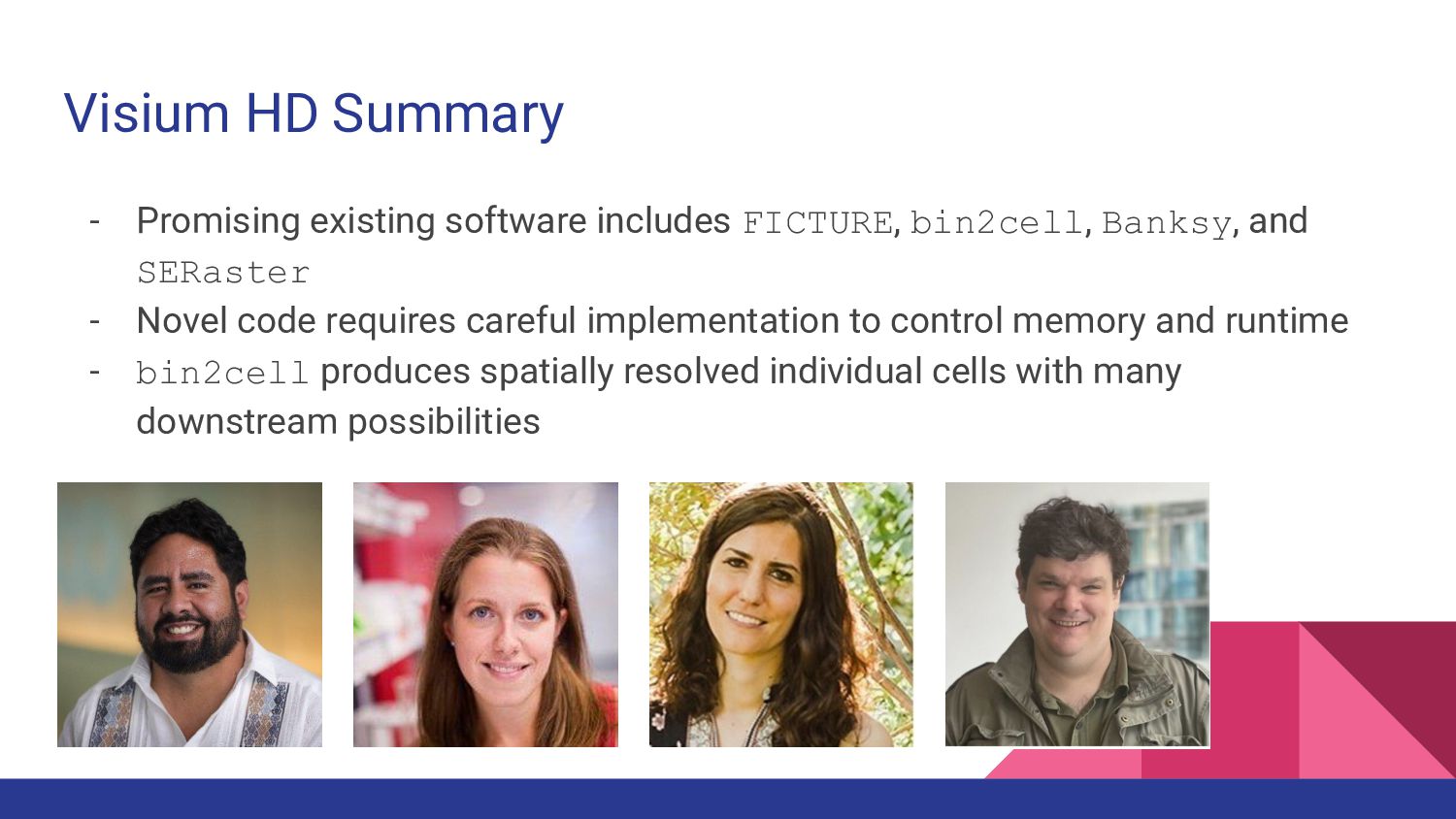
19. Visium HD Summary - Promising existing software includes FICTURE, bin2cell, Banksy, and SERaster - Novel code requires careful implementation to control memory and runtime - bin2cell produces spatially resolved individual cells with many downstream possibilities
20. sc/snRNA-seq data analysis Presented By Melissa Mayén Quiroz
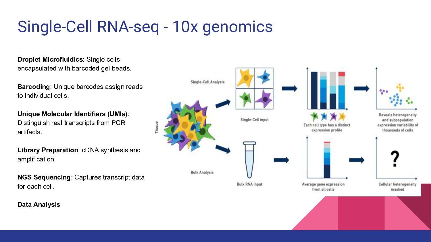
21. Droplet Microfluidics: Single cells encapsulated with barcoded gel beads. Barcoding: Unique barcodes assign reads to individual cells. Unique Molecular Identifiers (UMIs): Distinguish real transcripts from PCR artifacts. Library Preparation: cDNA synthesis and amplification. NGS Sequencing: Captures transcript data for each cell. Data Analysis Single-Cell RNA-seq - 10x genomics
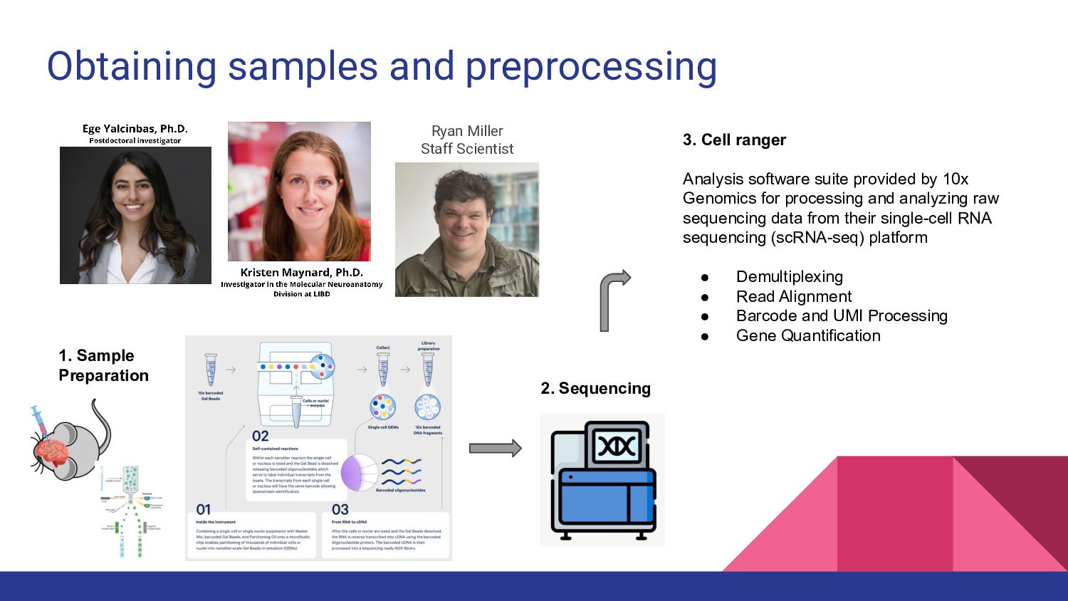
22. Obtaining samples and preprocessing Ryan Miller Staff Scientist 3. Cell ranger Analysis software suite provided by 10x Genomics for processing and analyzing raw sequencing data from their single-cell RNA sequencing (scRNA-seq) platform • Demultiplexing • Read Alignment • Barcode and UMI Processing • Gene Quantification 1. Sample Preparation 2. Sequencing
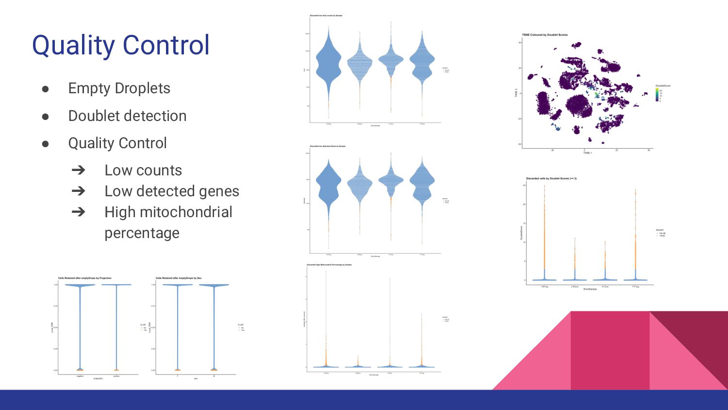
23. Quality Control • Empty Droplets • Doublet detection • Quality Control ➔ Low counts ➔ Low detected genes ➔ High mitochondrial percentage
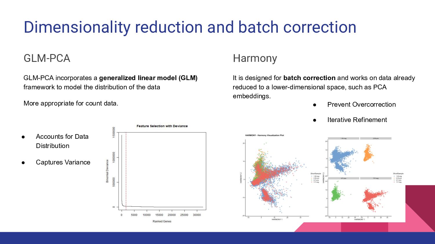
24. Dimensionality reduction and batch correction GLM-PCA GLM-PCA incorporates a generalized linear model (GLM) framework to model the distribution of the data More appropriate for count data. • Accounts for Data Distribution • Captures Variance Harmony It is designed for batch correction and works on data already reduced to a lower-dimensional space, such as PCA embeddings. • Prevent Overcorrection • Iterative Refinement
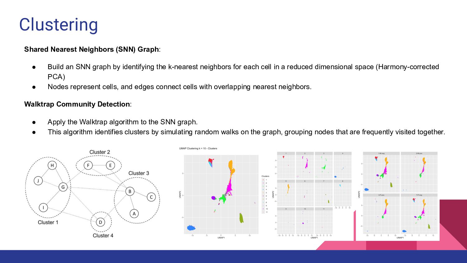
25. Clustering Shared Nearest Neighbors (SNN) Graph: • Build an SNN graph by identifying the k-nearest neighbors for each cell in a reduced dimensional space (Harmony-corrected PCA) • Nodes represent cells, and edges connect cells with overlapping nearest neighbors. Walktrap Community Detection: • Apply the Walktrap algorithm to the SNN graph. • This algorithm identifies clusters by simulating random walks on the graph, grouping nodes that are frequently visited together.
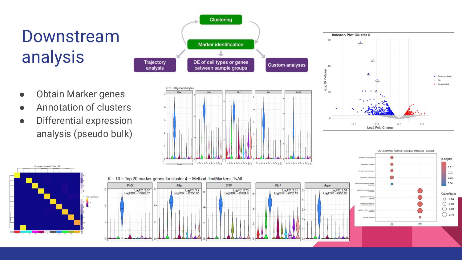
26. Downstream analysis • Obtain Marker genes • Annotation of clusters • Differential expression analysis (pseudo bulk)
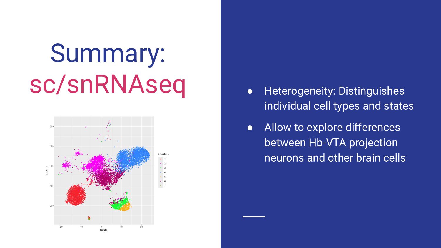
27. Summary: sc/snRNAseq • Heterogeneity: Distinguishes individual cell types and states • Allow to explore differences between Hb-VTA projection neurons and other brain cells
28. Multi-ome data analysis (snATAC-seq + snRNA-seq) Presented By Cynthia Soto Cardinault
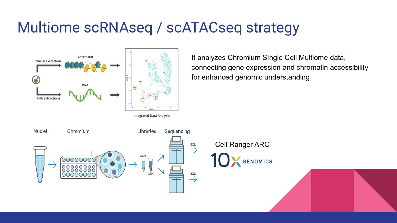
29. Multiome scRNAseq / scATACseq strategy It analyzes Chromium Single Cell Multiome data, connecting gene expression and chromatin accessibility for enhanced genomic understanding Cell Ranger ARC
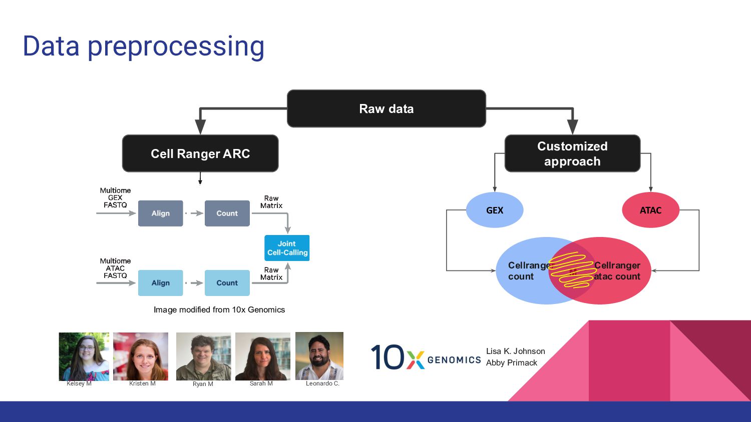
30. Data preprocessing Raw data Ryan M Kristen M Sarah M Kelsey M Leonardo C. Customized approach Cellranger count M GEX ATAC Cellranger atac count Lisa K. Johnson Abby Primack Cell Ranger ARC Image modified from 10x Genomics
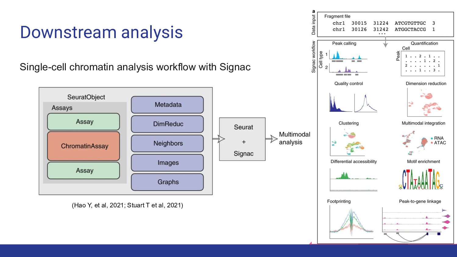
31. Downstream analysis (Hao Y, et al, 2021; Stuart T et al, 2021) Single-cell chromatin analysis workflow with Signac
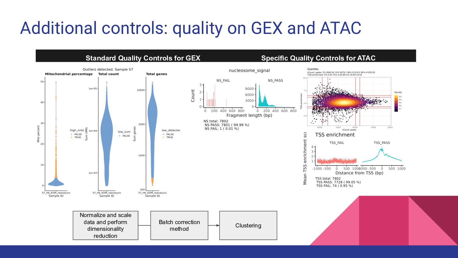
32. Additional controls: quality on GEX and ATAC Standard Quality Controls for GEX Specific Quality Controls for ATAC Normalize and scale data and perform dimensionality reduction Batch correction method Clustering
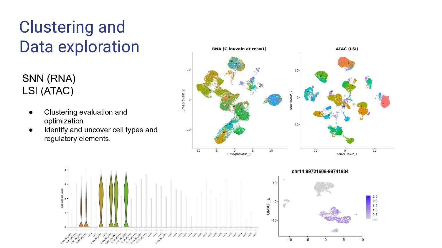
33. Clustering and Data exploration • Clustering evaluation and optimization • Identify and uncover cell types and regulatory elements. SNN (RNA) LSI (ATAC)
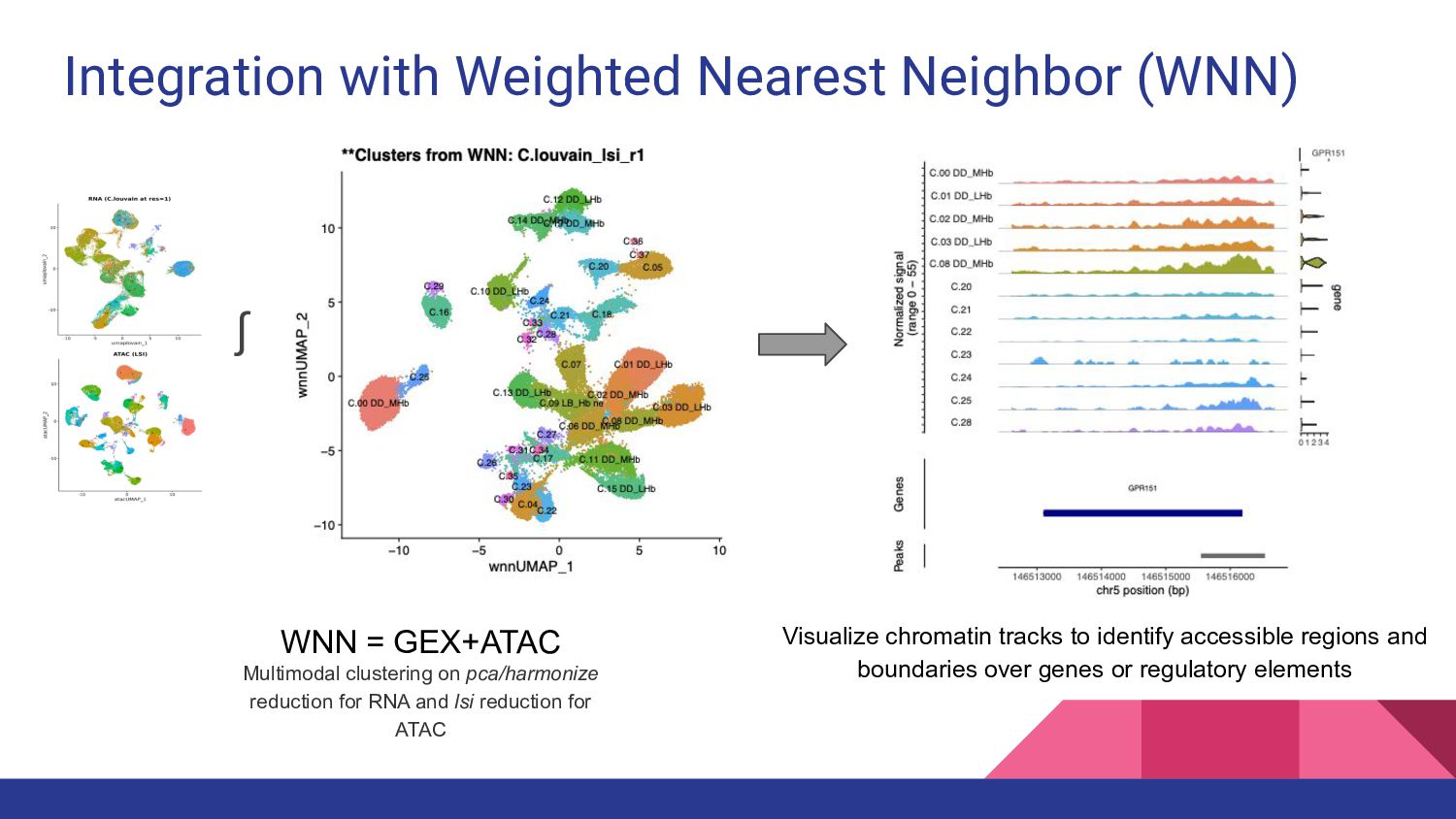
34. Integration with Weighted Nearest Neighbor (WNN) WNN = GEX+ATAC Multimodal clustering on pca/harmonize reduction for RNA and lsi reduction for ATAC ∫ Visualize chromatin tracks to identify accessible regions and boundaries over genes or regulatory elements
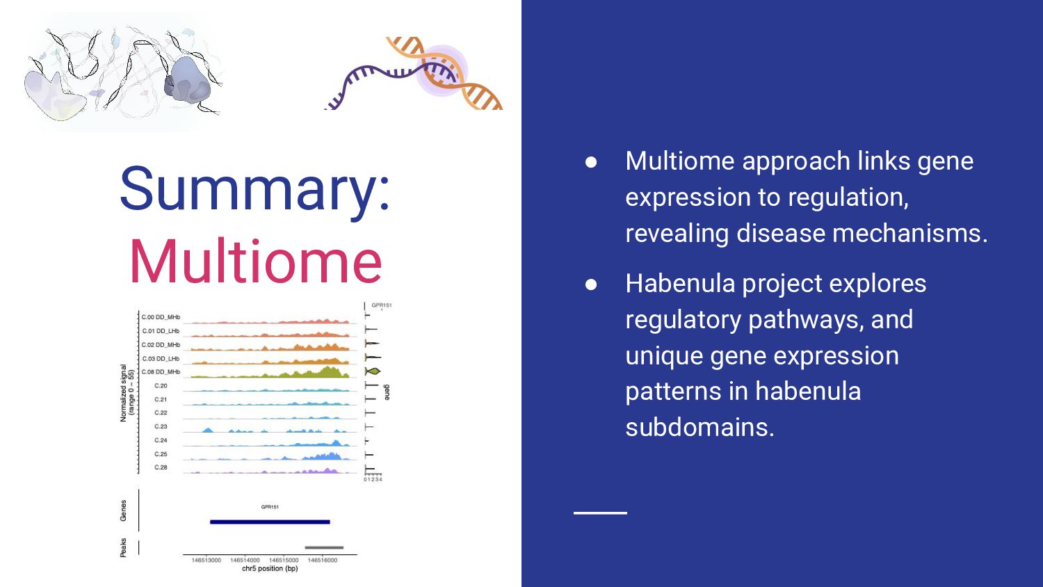
35. Summary: Multiome • Multiome approach links gene expression to regulation, revealing disease mechanisms. • Habenula project explores regulatory pathways, and unique gene expression patterns in habenula subdomains.
36. Bulk RNA-seq deconvolution Presented By Louise Huuki-Myers
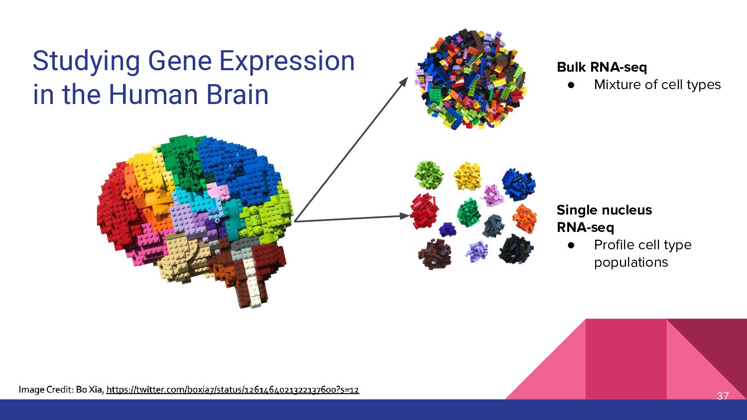
37. Studying Gene Expression in the Human Brain Bulk RNA-seq • Mixture of cell types Single nucleus RNA-seq • Profile cell type populations 37
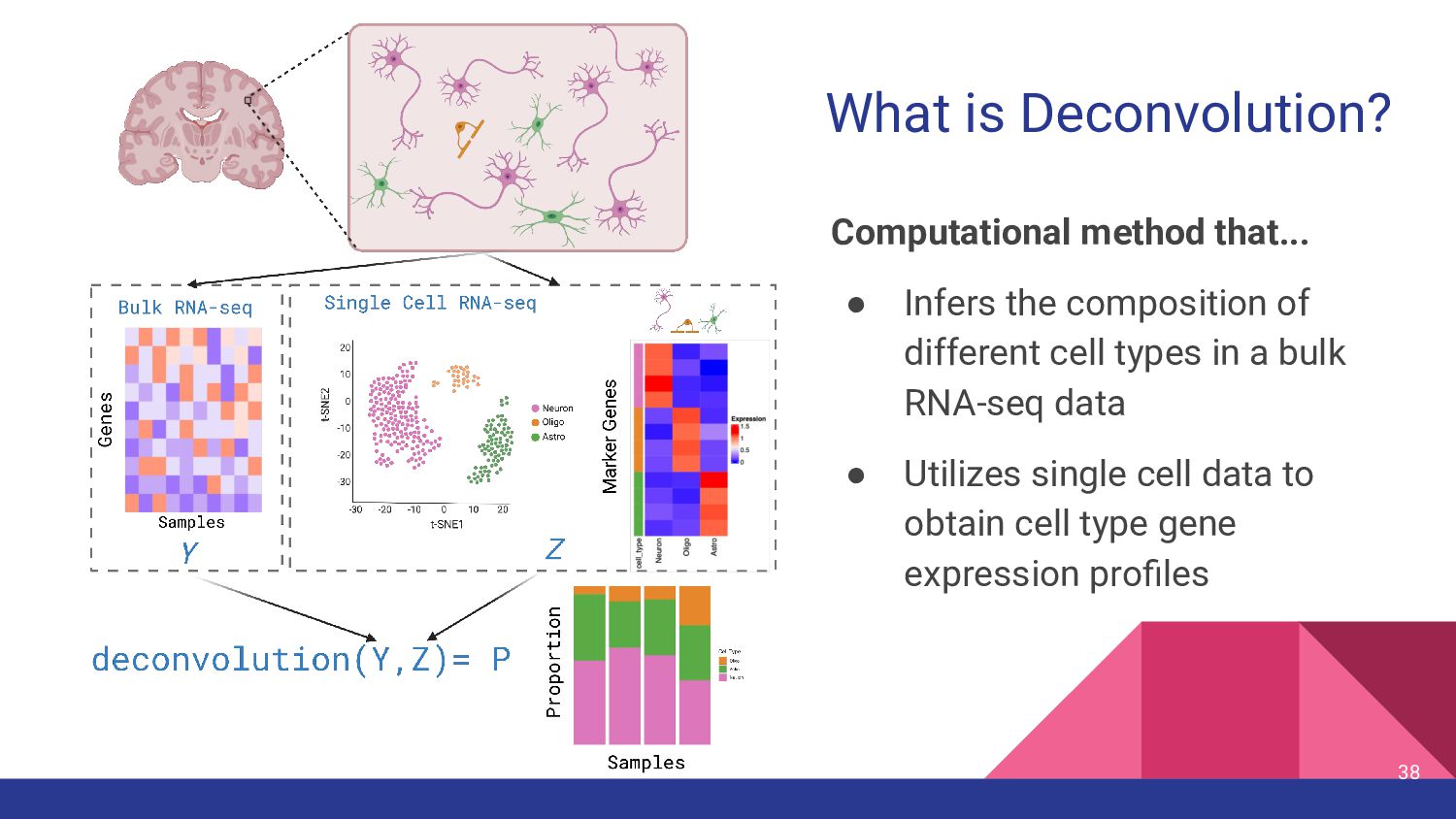
38. What is Deconvolution? Computational method that... • Infers the composition of different cell types in a bulk RNA-seq data • Utilizes single cell data to obtain cell type gene expression profiles 38
39. Mean Ratio Gene Selection DeconvoBuddies::get_mean_ratio2()
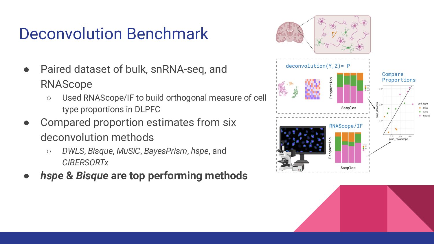
40. Deconvolution Benchmark • Paired dataset of bulk, snRNA-seq, and RNAScope ◦ Used RNAScope/IF to build orthogonal measure of cell type proportions in DLPFC • Compared proportion estimates from six deconvolution methods ◦ DWLS, Bisque, MuSiC, BayesPrism, hspe, and CIBERSORTx • hspe & Bisque are top performing methods
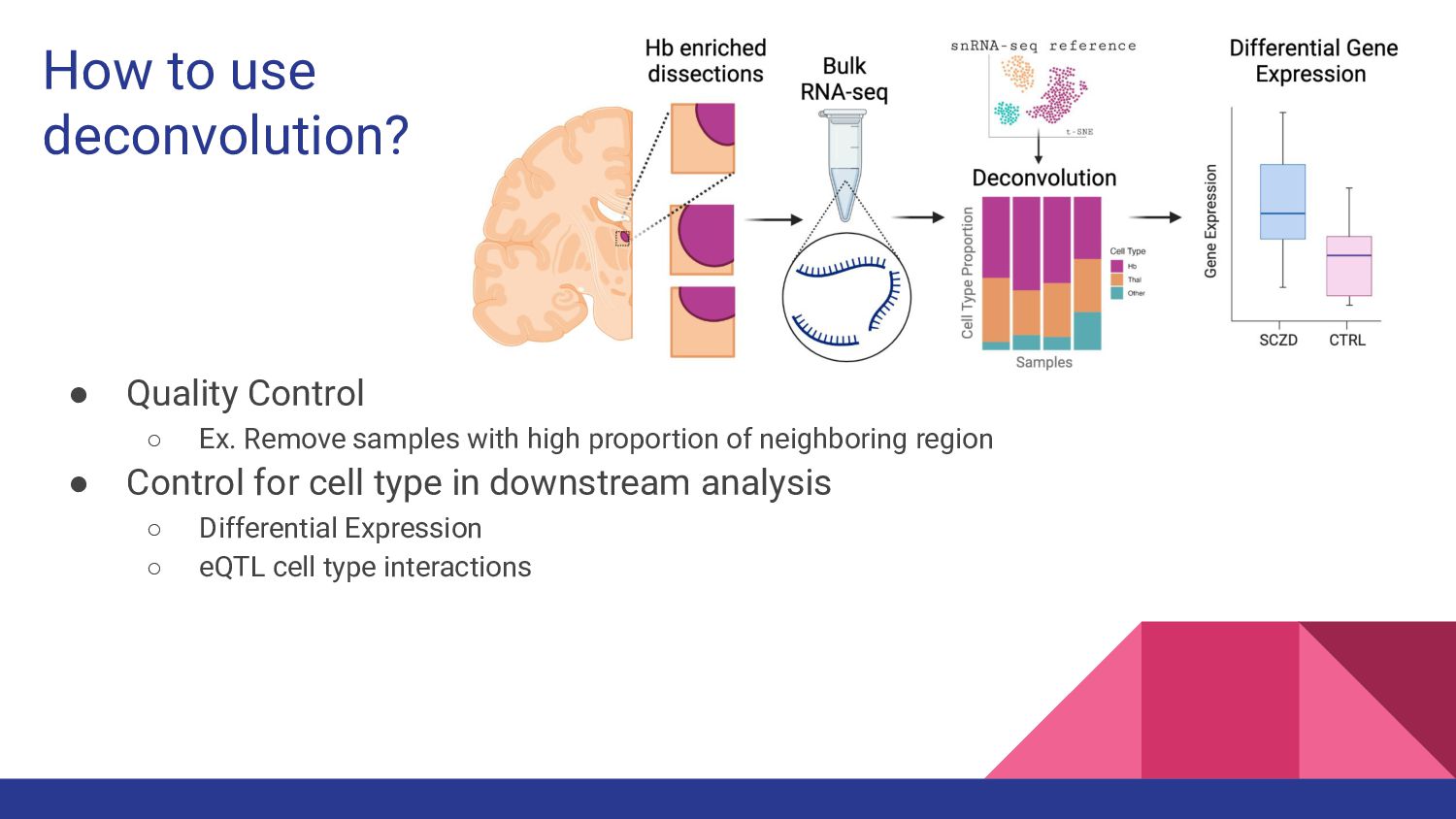
41. • Quality Control ◦ Ex. Remove samples with high proportion of neighboring region • Control for cell type in downstream analysis ◦ Differential Expression ◦ eQTL cell type interactions How to use deconvolution?
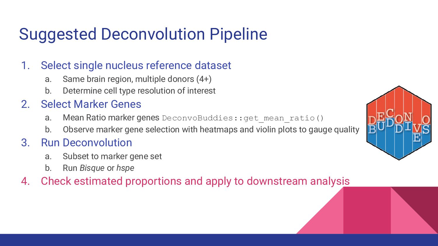
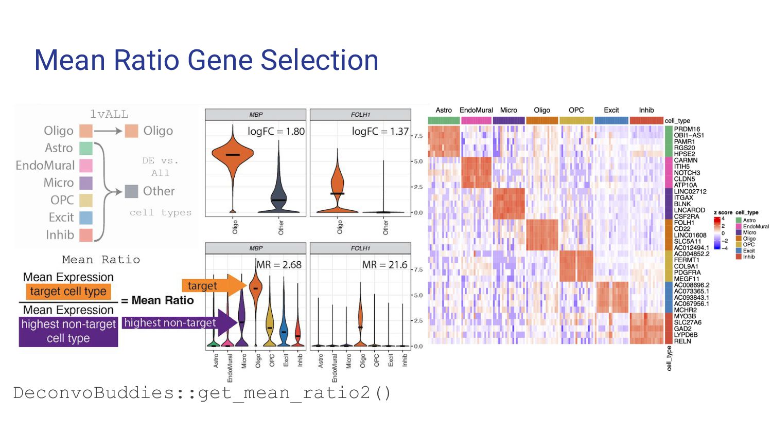
42. Suggested Deconvolution Pipeline 1. Select single nucleus reference dataset a. Same brain region, multiple donors (4+) b. Determine cell type resolution of interest 2. Select Marker Genes a. Mean Ratio marker genes DeconvoBuddies::get_mean_ratio() b. Observe marker gene selection with heatmaps and violin plots to gauge quality 3. Run Deconvolution a. Subset to marker gene set b. Run Bisque or hspe 4. Check estimated proportions and apply to downstream analysis
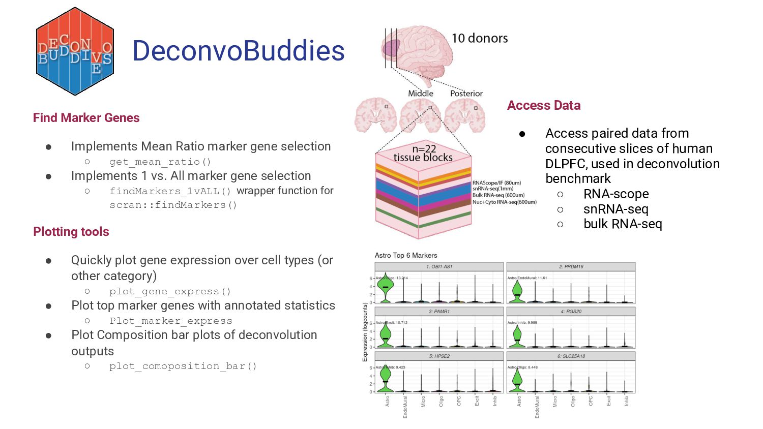
43. DeconvoBuddies Find Marker Genes • Implements Mean Ratio marker gene selection ◦ get_mean_ratio() • Implements 1 vs. All marker gene selection ◦ findMarkers_1vALL() wrapper function for scran::findMarkers() Plotting tools • Quickly plot gene expression over cell types (or other category) ◦ plot_gene_express() • Plot top marker genes with annotated statistics ◦ Plot_marker_express • Plot Composition bar plots of deconvolution outputs ◦ plot_comoposition_bar() Access Data • Access paired data from consecutive slices of human DLPFC, used in deconvolution benchmark ◦ RNA-scope ◦ snRNA-seq ◦ bulk RNA-seq
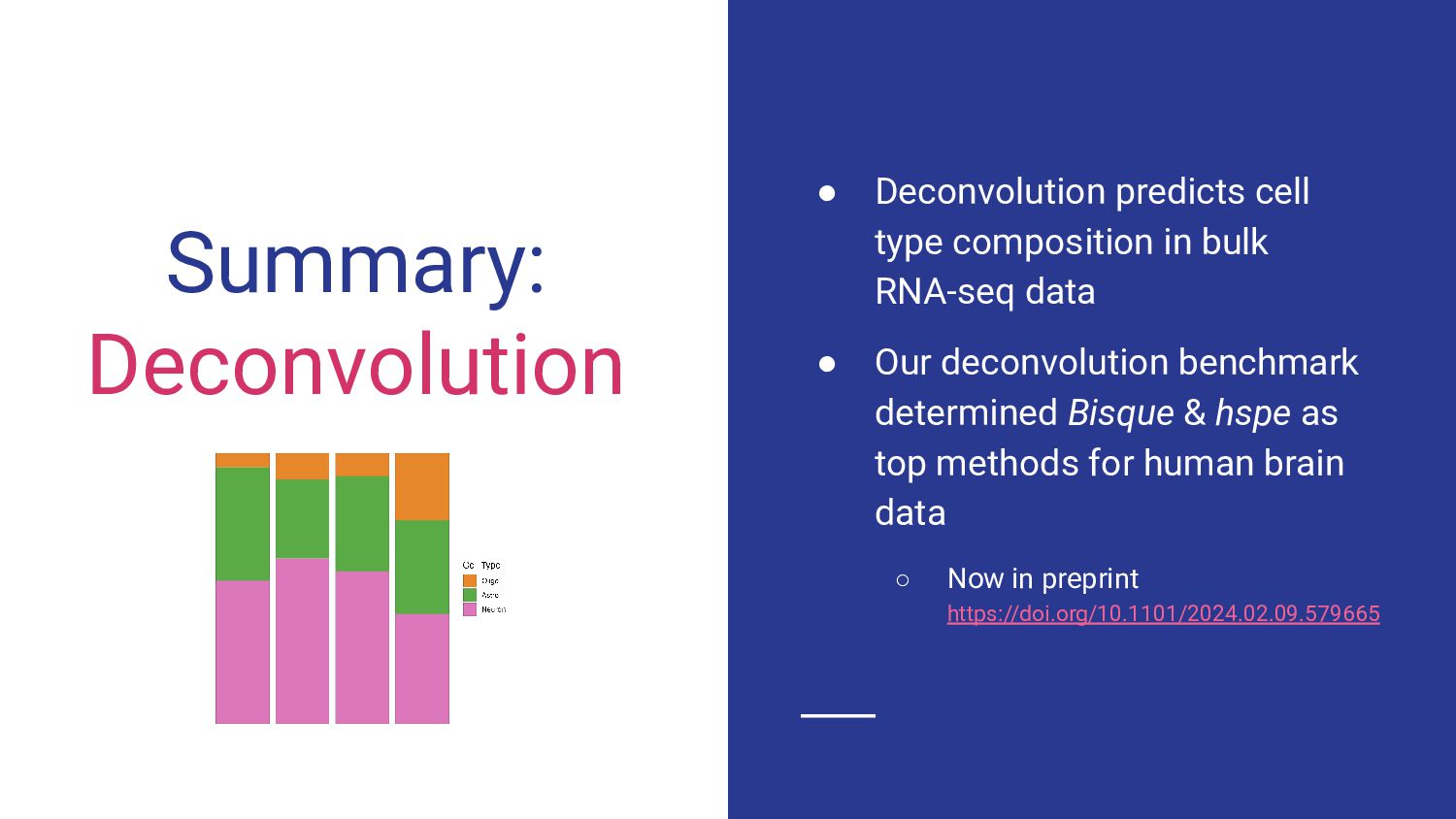
44. Summary: Deconvolution • Deconvolution predicts cell type composition in bulk RNA-seq data • Our deconvolution benchmark determined Bisque & hspe as top methods for human brain data ◦ Now in preprint https://doi.org/10.1101/2024.02.09.579665
45. Bulk RNA-seq data analysis
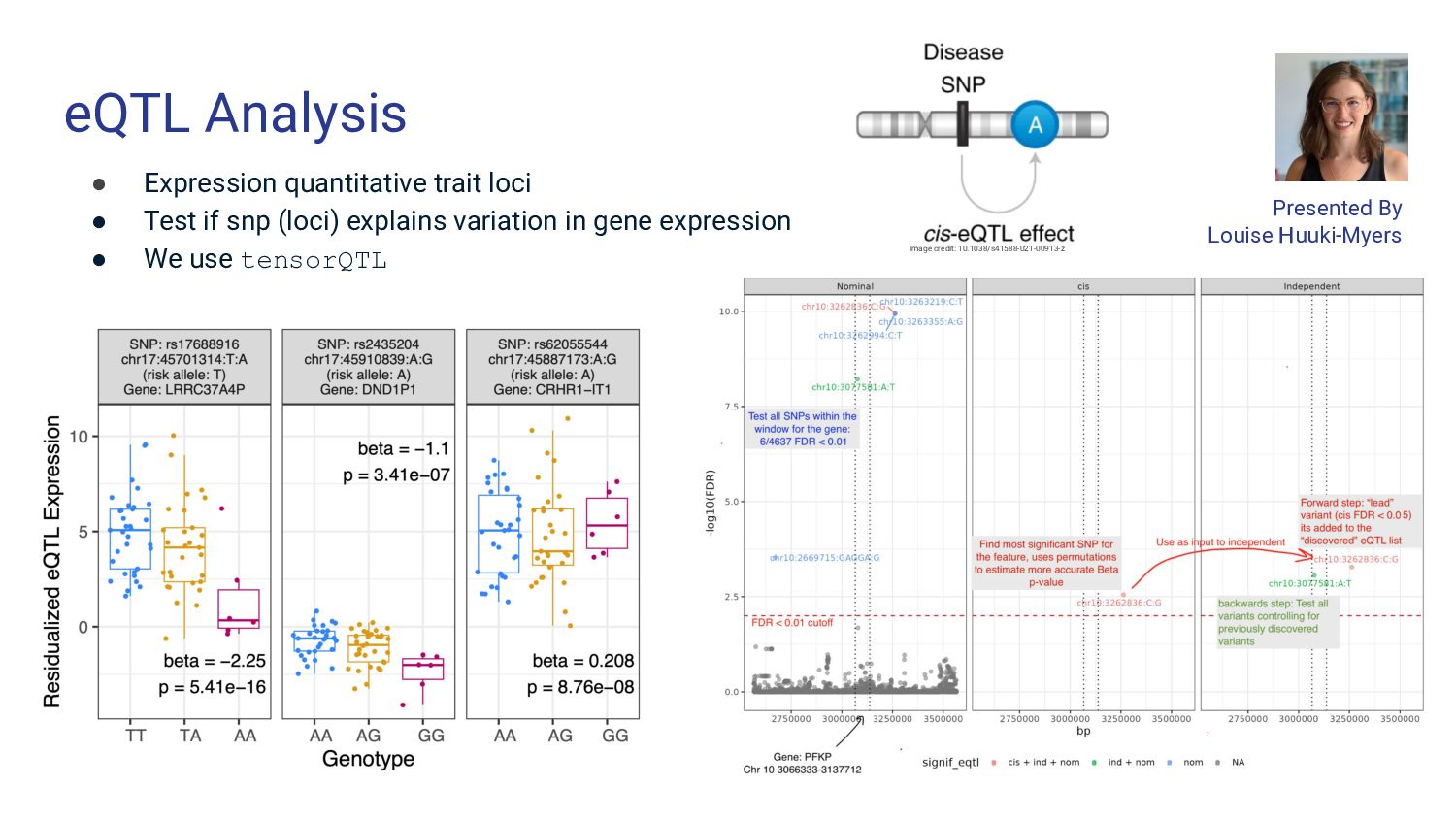
46. eQTL Analysis • Expression quantitative trait loci • Test if snp (loci) explains variation in gene expression • We use tensorQTL Presented By Louise Huuki-Myers Image credit: 10.1038/s41588-021-00913-z
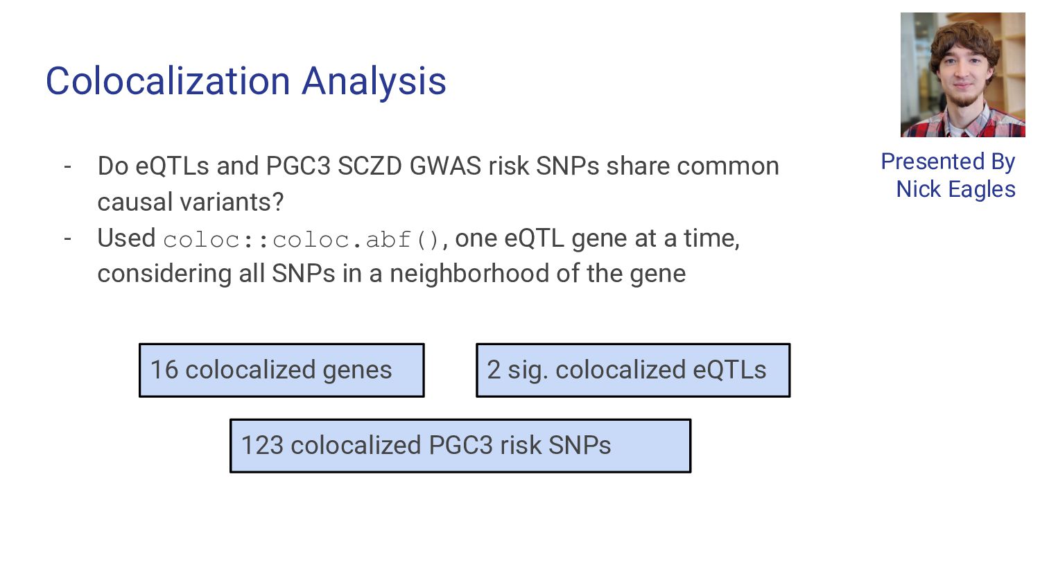
47. - Do eQTLs and PGC3 SCZD GWAS risk SNPs share common causal variants? - Used coloc::coloc.abf(), one eQTL gene at a time, considering all SNPs in a neighborhood of the gene Colocalization Analysis Presented By Nick Eagles 16 colocalized genes 2 sig. colocalized eQTLs 123 colocalized PGC3 risk SNPs
48. qsvaR Presented By Nick Eagles
49. qsvaR Background - Post-mortem studies involve a post-mortem interval where tissue degrades before being frozen - Different transcripts degrade at different rates - Degradation confounds biological signal in differential expression analysis and can produce false positives
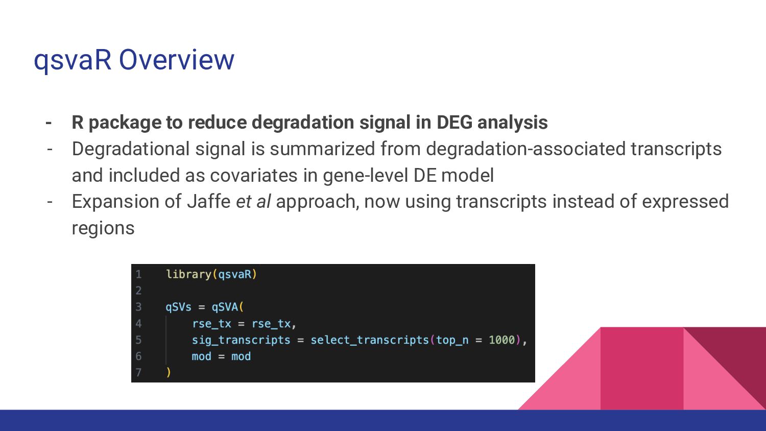
50. qsvaR Overview - R package to reduce degradation signal in DEG analysis - Degradational signal is summarized from degradation-associated transcripts and included as covariates in gene-level DE model - Expansion of Jaffe et al approach, now using transcripts instead of expressed regions
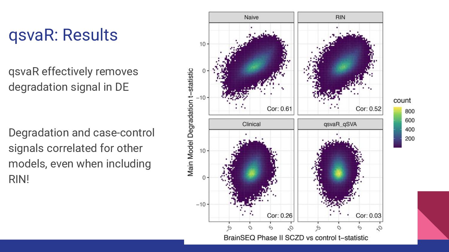
51. qsvaR: Results qsvaR effectively removes degradation signal in DE Degradation and case-control signals correlated for other models, even when including RIN!
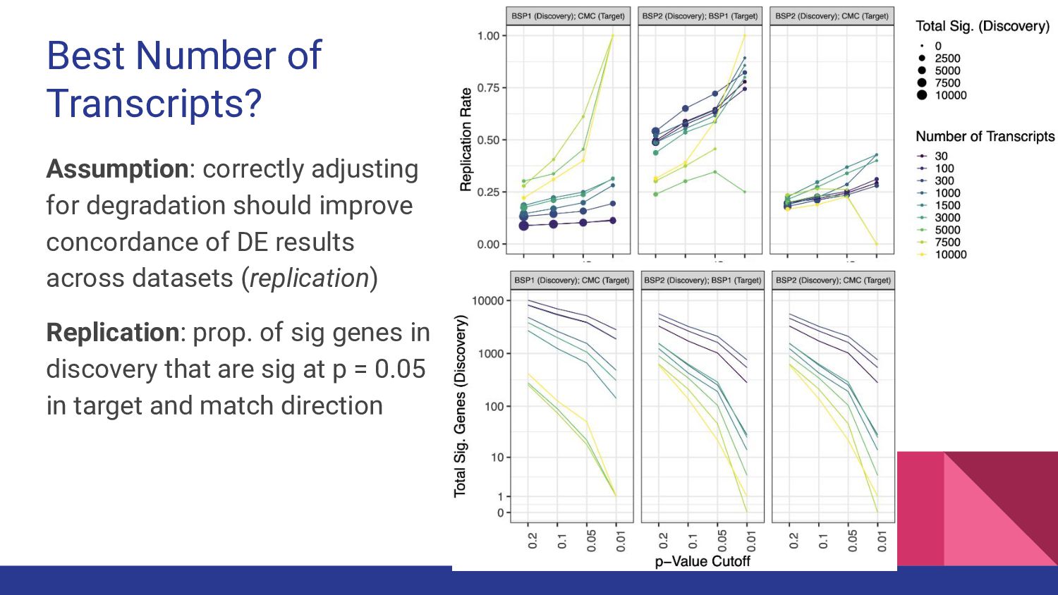
52. Best Number of Transcripts? Assumption: correctly adjusting for degradation should improve concordance of DE results across datasets (replication) Replication: prop. of sig genes in discovery that are sig at p = 0.05 in target and match direction
53. Summary: qsvaR • qsvaR is an R package reducing the confounding effect of degradation on DE • Requires transcript-level data instead of expressed regions • Upcoming manuscript
54. CHESS-Brain Presented By Geo Pertea
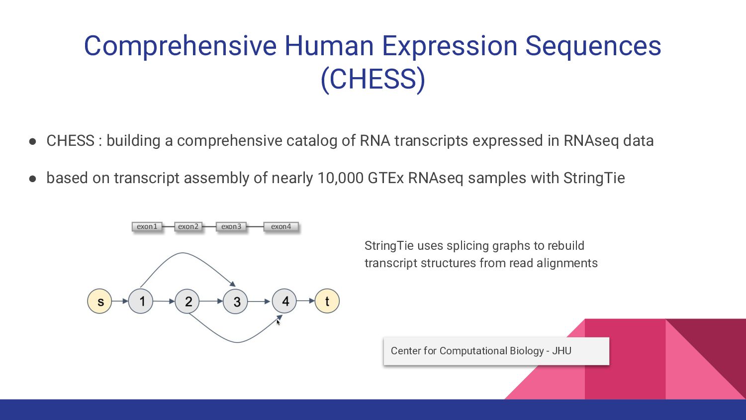
55. Center for Computational Biology - JHU • CHESS : building a comprehensive catalog of RNA transcripts expressed in RNAseq data • based on transcript assembly of nearly 10,000 GTEx RNAseq samples with StringTie Comprehensive Human Expression Sequences (CHESS) exon2 exon3 exon1 exon4 StringTie uses splicing graphs to rebuild transcript structures from read alignments
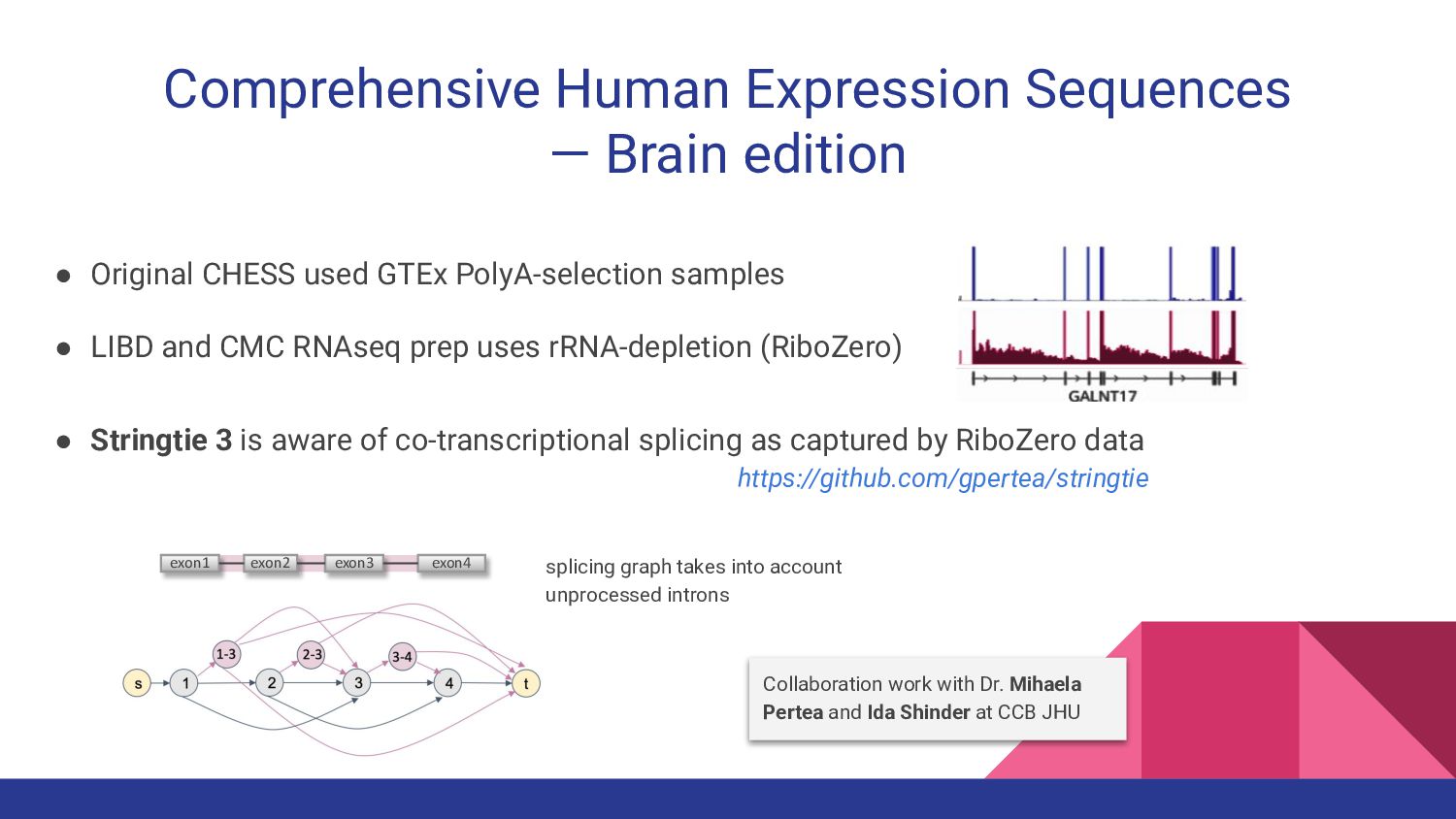
56. Collaboration work with Dr. Mihaela Pertea and Ida Shinder at CCB JHU • Original CHESS used GTEx PolyA-selection samples • LIBD and CMC RNAseq prep uses rRNA-depletion (RiboZero) • Stringtie 3 is aware of co-transcriptional splicing as captured by RiboZero data Comprehensive Human Expression Sequences — Brain edition exon2 exon3 exon1 exon4 splicing graph takes into account unprocessed introns https://github.com/gpertea/stringtie
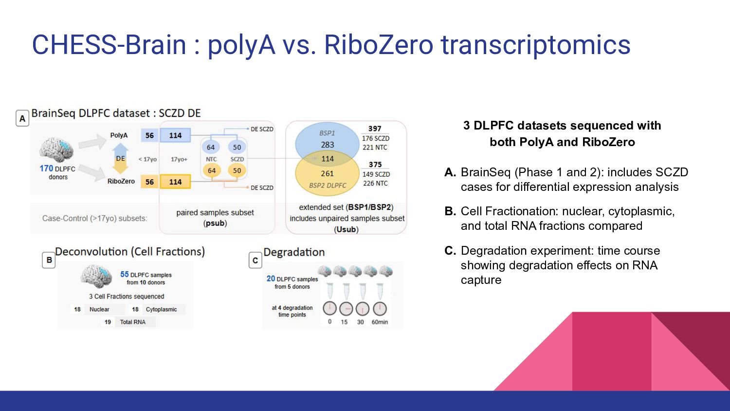
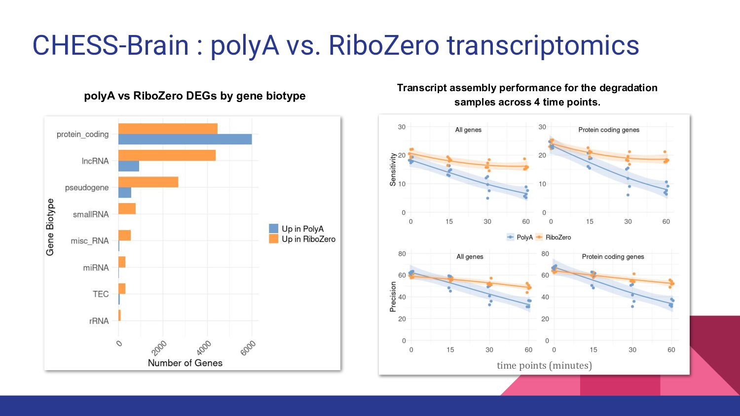
57. CHESS-Brain : polyA vs. RiboZero transcriptomics A. BrainSeq (Phase 1 and 2): includes SCZD cases for differential expression analysis B. Cell Fractionation: nuclear, cytoplasmic, and total RNA fractions compared C. Degradation experiment: time course showing degradation effects on RNA capture 3 DLPFC datasets sequenced with both PolyA and RiboZero
58. CHESS-Brain : polyA vs. RiboZero transcriptomics Transcript assembly performance for the degradation samples across 4 time points. time points (minutes) polyA vs RiboZero DEGs by gene biotype
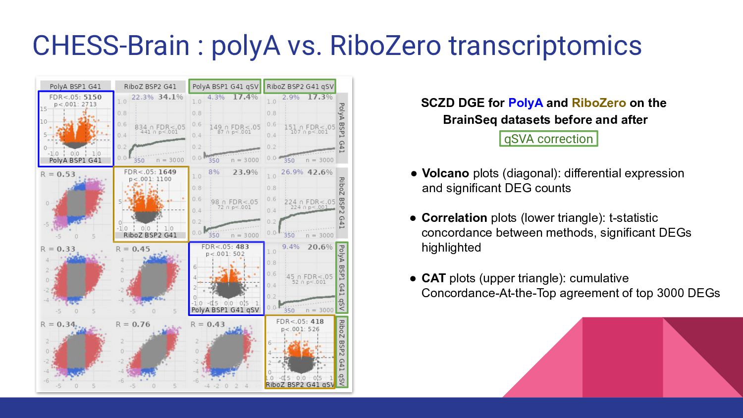
59. SCZD DGE for PolyA and RiboZero on the BrainSeq datasets before and after • Volcano plots (diagonal): differential expression and significant DEG counts CHESS-Brain : polyA vs. RiboZero transcriptomics • Correlation plots (lower triangle): t-statistic concordance between methods, significant DEGs highlighted • CAT plots (upper triangle): cumulative Concordance-At-the-Top agreement of top 3000 DEGs qSVA correction
60. Summary: CHESS-Brain • Data-driven expansion of the catalog of RNA transcripts expressed in brain tissue • Improved transcript-level analyses of LIBD RNAseq RiboZero data • Upcoming manuscripts
61. Open source software development Presented By Nick Eagles
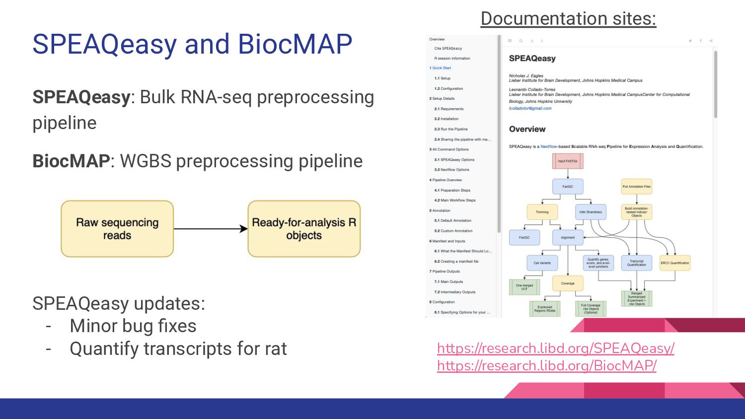
62. SPEAQeasy and BiocMAP SPEAQeasy: Bulk RNA-seq preprocessing pipeline BiocMAP: WGBS preprocessing pipeline Documentation sites: https://research.libd.org/SPEAQeasy/ https://research.libd.org/BiocMAP/ SPEAQeasy updates: - Minor bug fixes - Quantify transcripts for rat
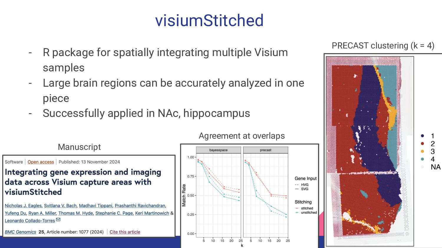
63. visiumStitched - R package for spatially integrating multiple Visium samples - Large brain regions can be accurately analyzed in one piece - Successfully applied in NAc, hippocampus Agreement at overlaps PRECAST clustering (k = 4) Manuscript
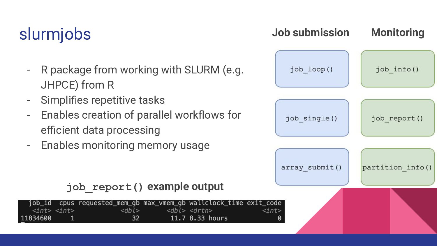
64. slurmjobs - R package from working with SLURM (e.g. JHPCE) from R - Simplifies repetitive tasks - Enables creation of parallel workflows for efficient data processing - Enables monitoring memory usage Job submission Monitoring job_report() example output
65. Packages Maintained by the Team • SpatialLIBD • DeconvoBuddies • qsvaR • SPEAQeasy • visiumStitched • slurmjobs
66. LIBD JHPCE Presented By Nick Eagles
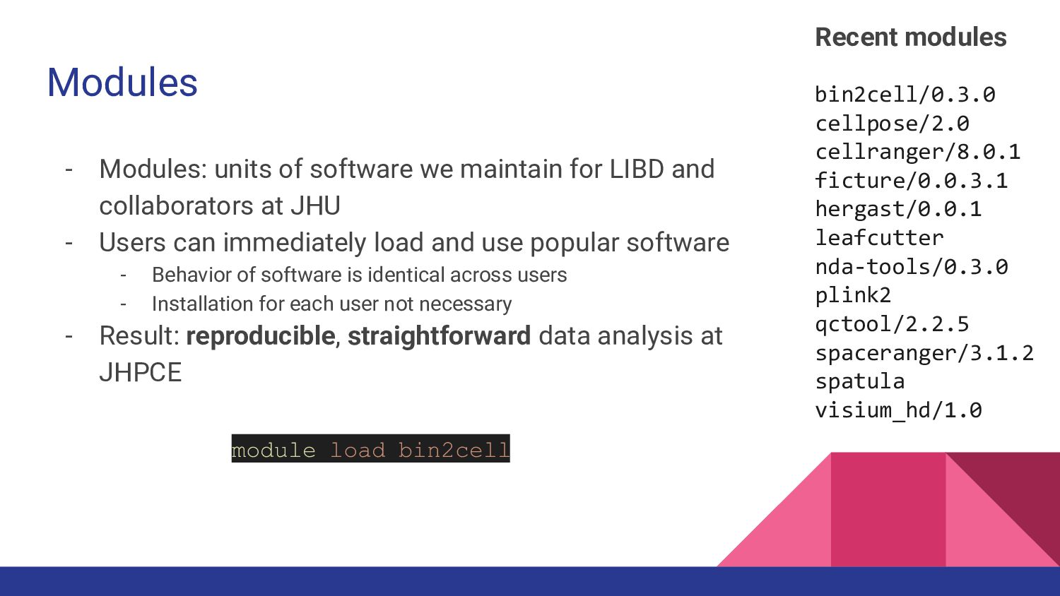
67. Modules - Modules: units of software we maintain for LIBD and collaborators at JHU - Users can immediately load and use popular software - Behavior of software is identical across users - Installation for each user not necessary - Result: reproducible, straightforward data analysis at JHPCE bin2cell/0.3.0 cellpose/2.0 cellranger/8.0.1 ficture/0.0.3.1 hergast/0.0.1 leafcutter nda-tools/0.3.0 plink2 qctool/2.2.5 spaceranger/3.1.2 spatula visium_hd/1.0 Recent modules module load bin2cell
68. LIBD rstats club + Journal club videos
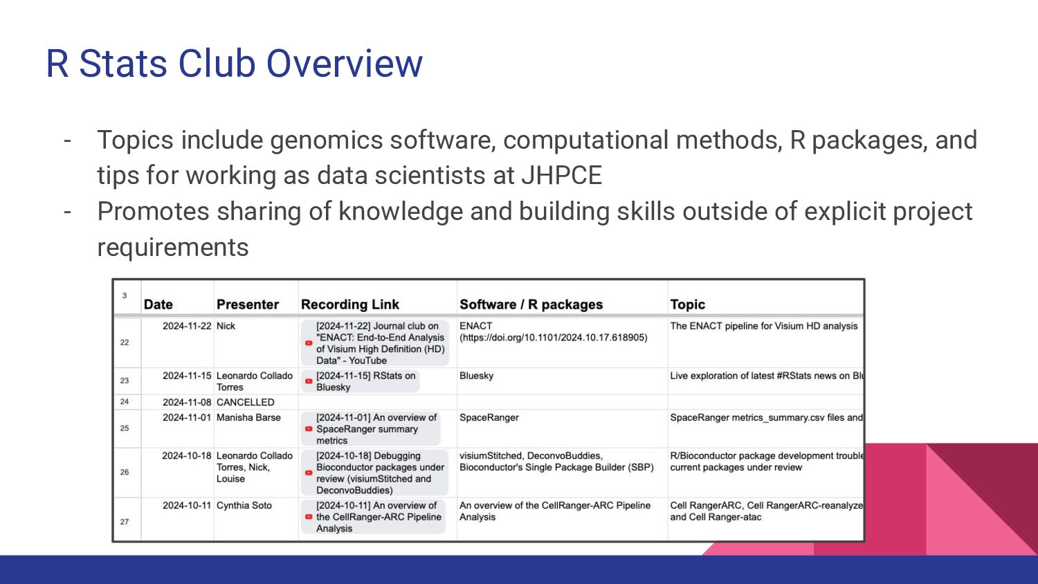
69. R Stats Club Overview - Topics include genomics software, computational methods, R packages, and tips for working as data scientists at JHPCE - Promotes sharing of knowledge and building skills outside of explicit project requirements
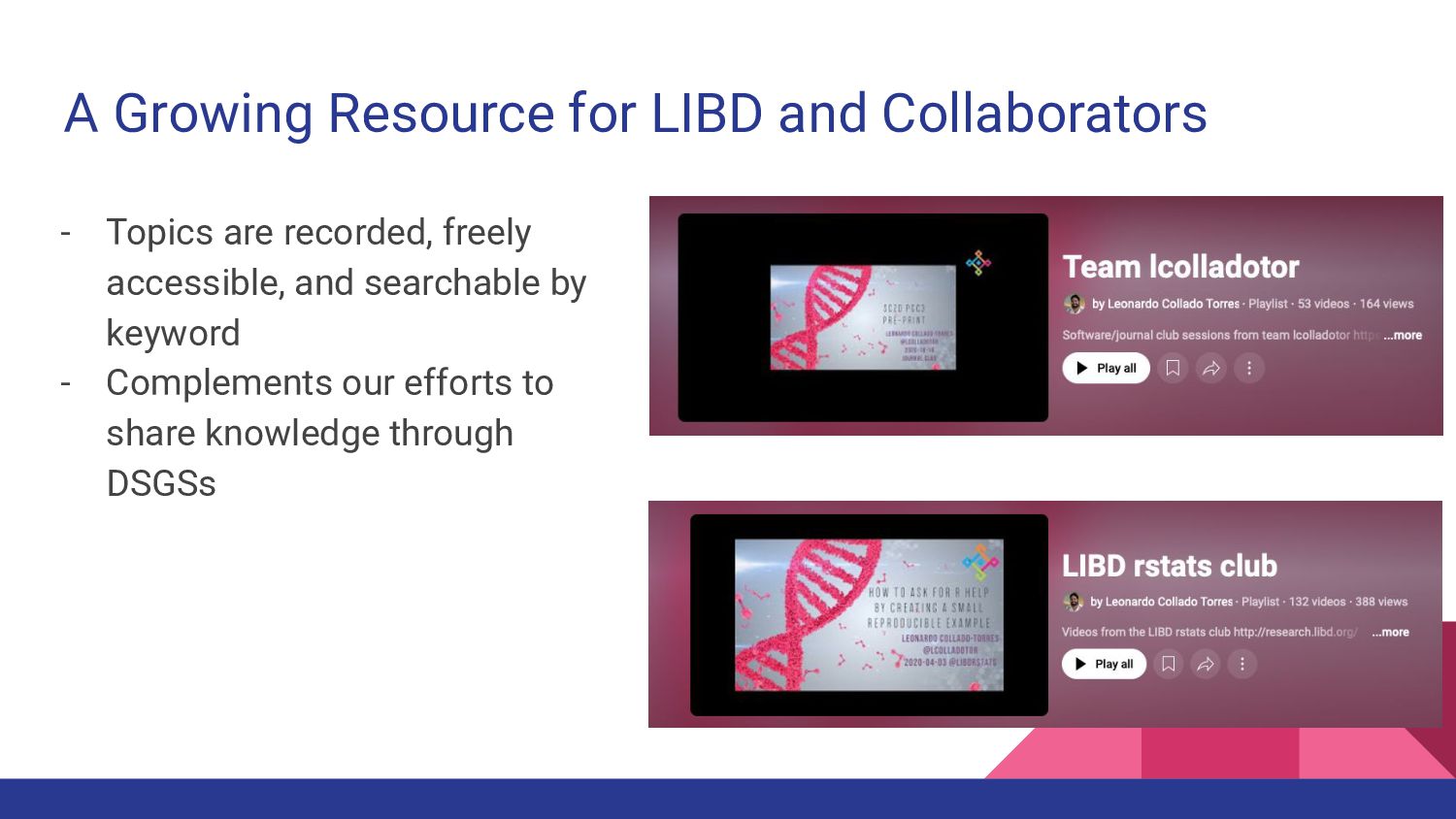
70. A Growing Resource for LIBD and Collaborators - Topics are recorded, freely accessible, and searchable by keyword - Complements our efforts to share knowledge through DSGSs
71. lcolladotor.github.io @lcolladotor.bsky.social Slides: