Using Electromagnetics to Delineate the Distribution of Proppant in a Hydraulically Fractured Reservoir

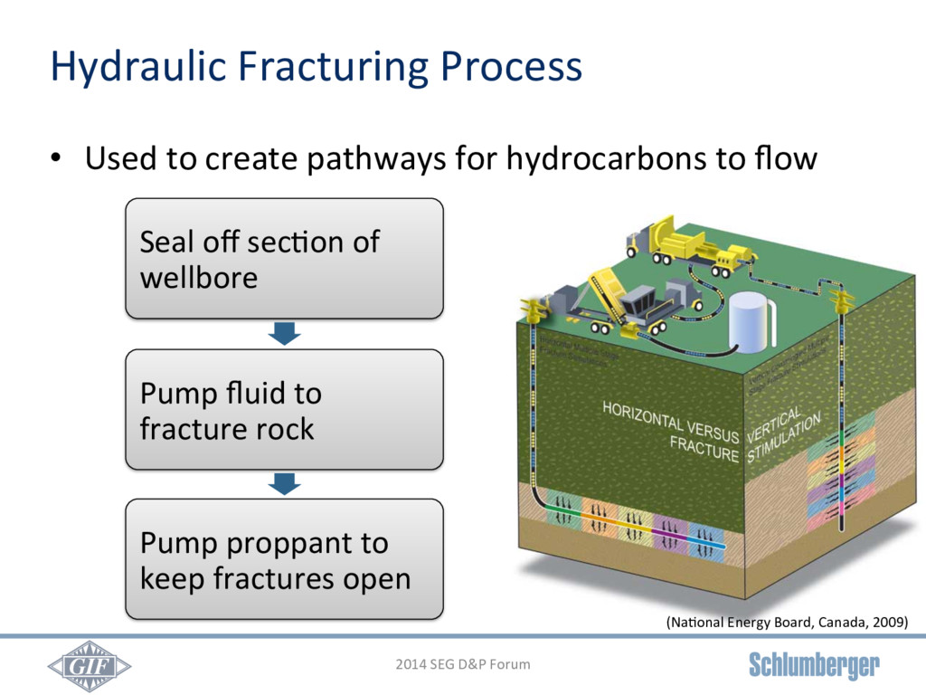
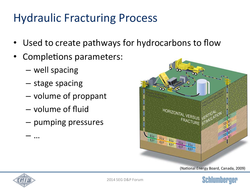
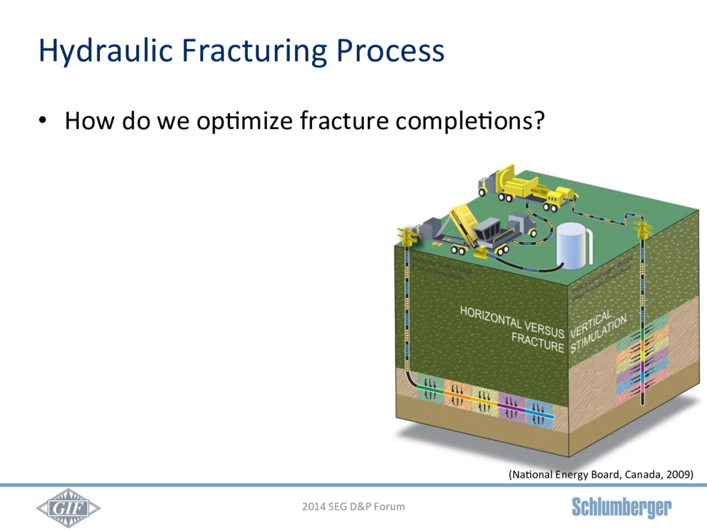
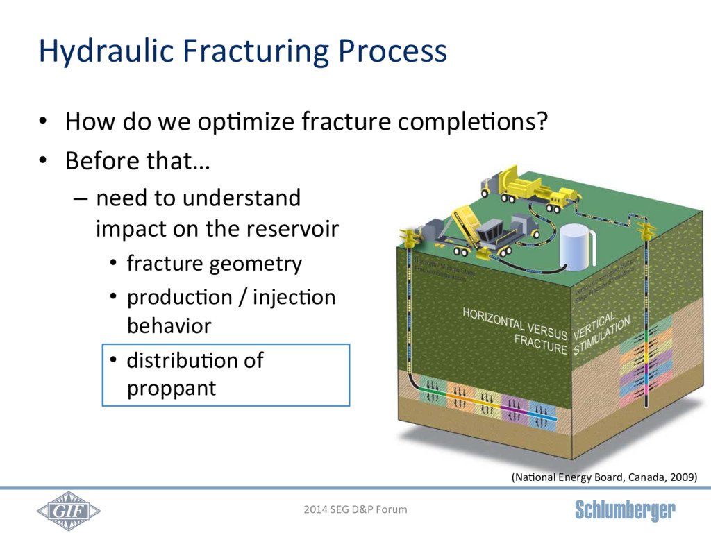
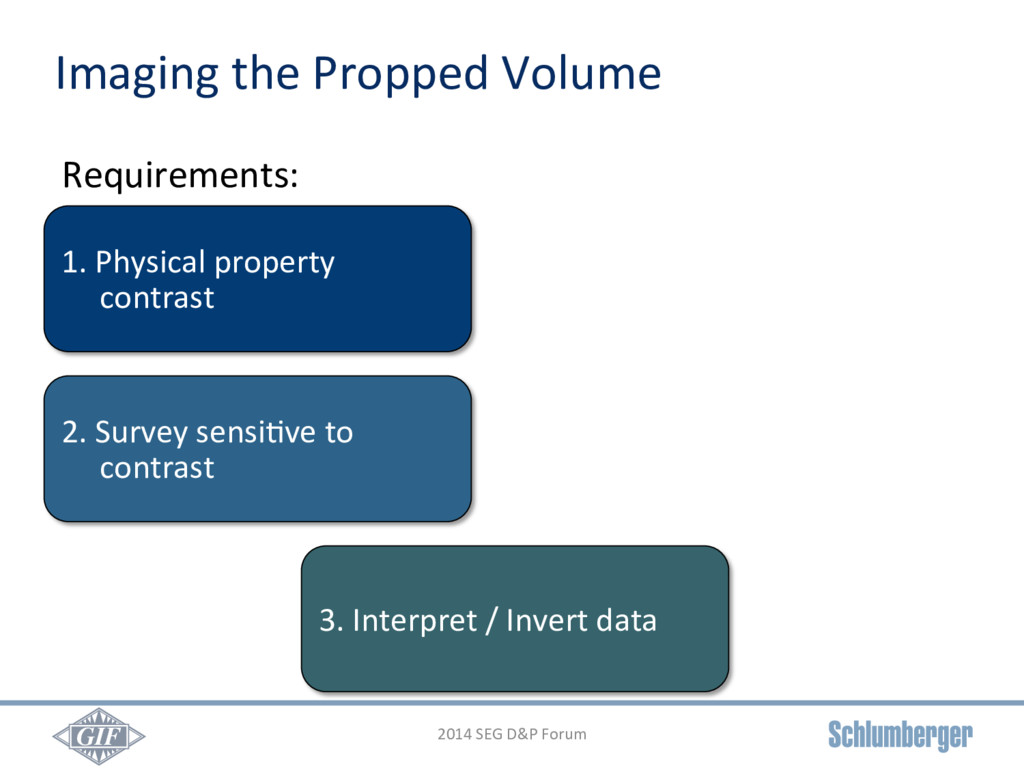
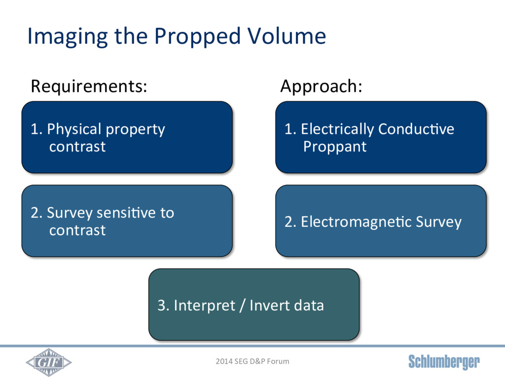
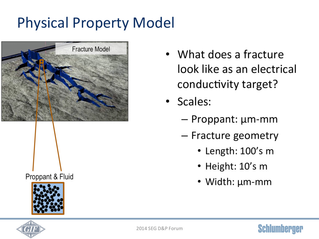
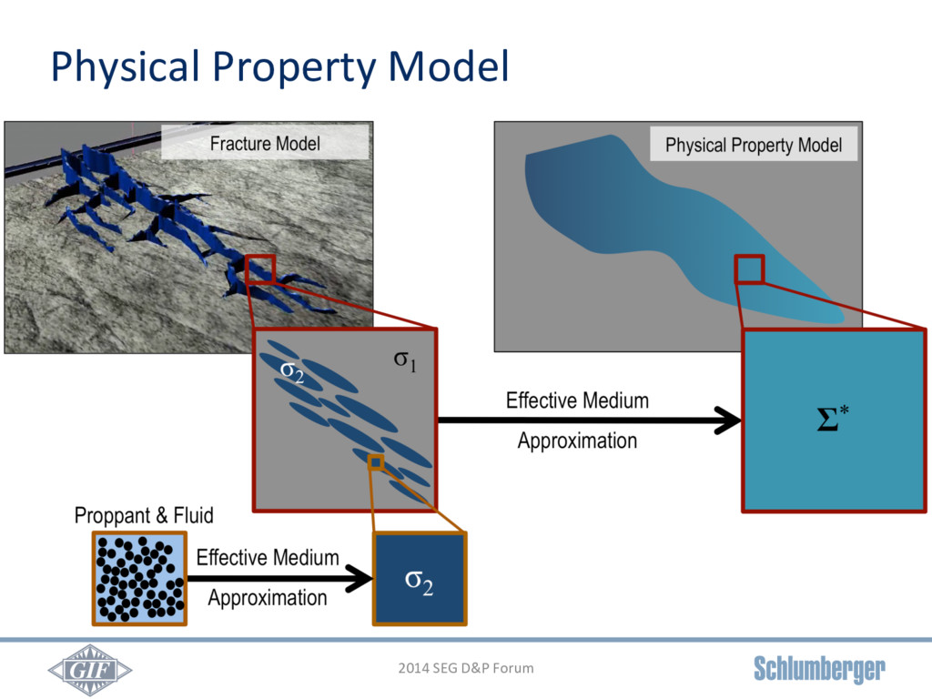
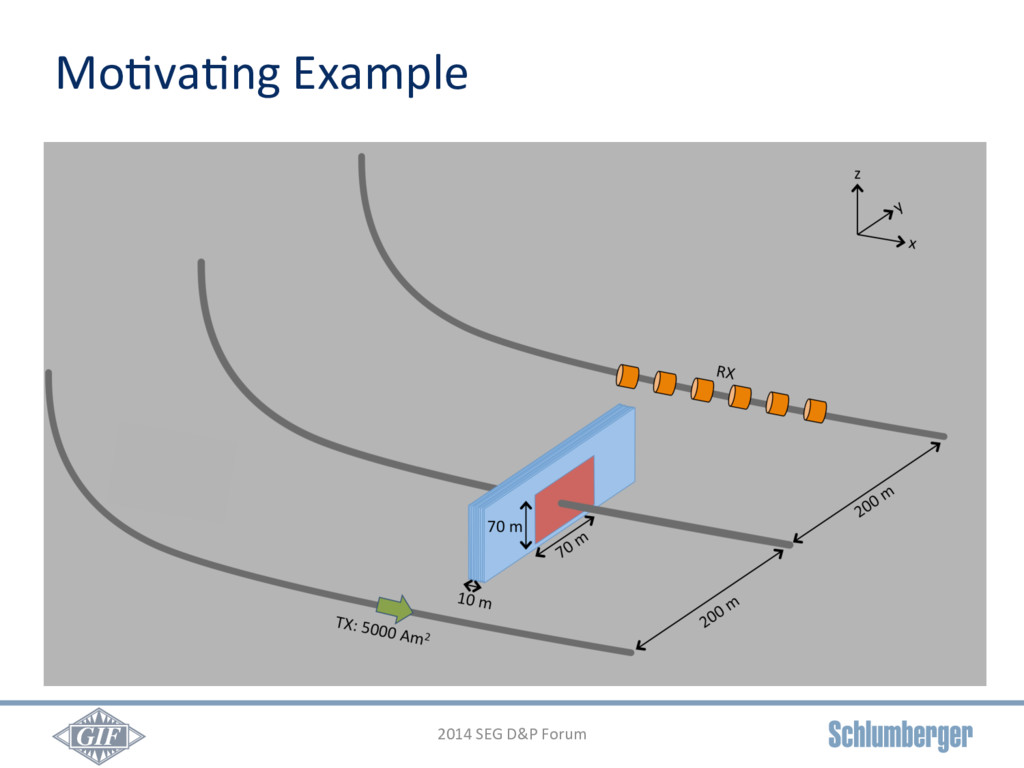
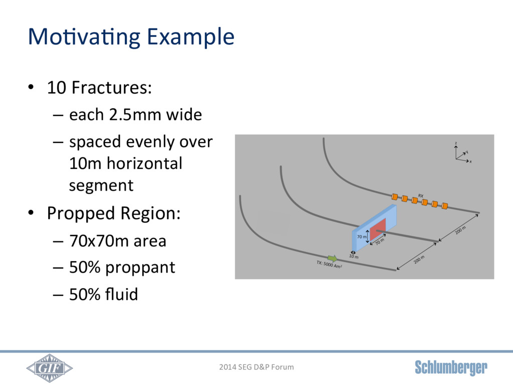
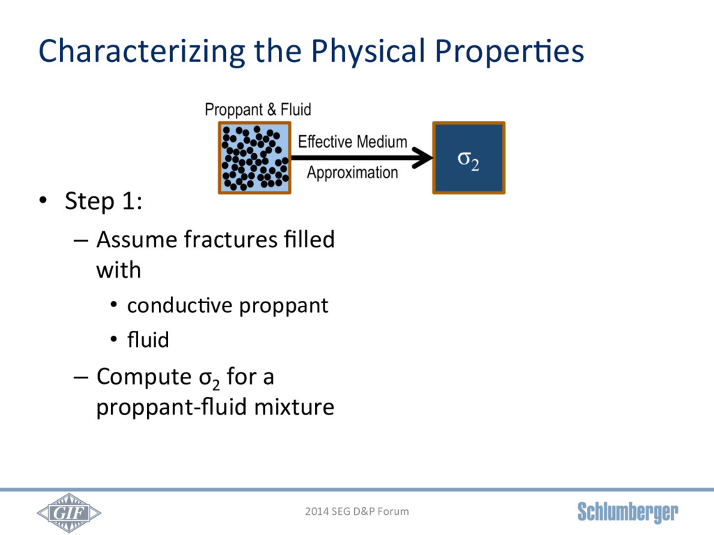
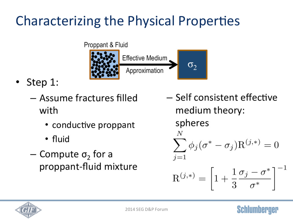
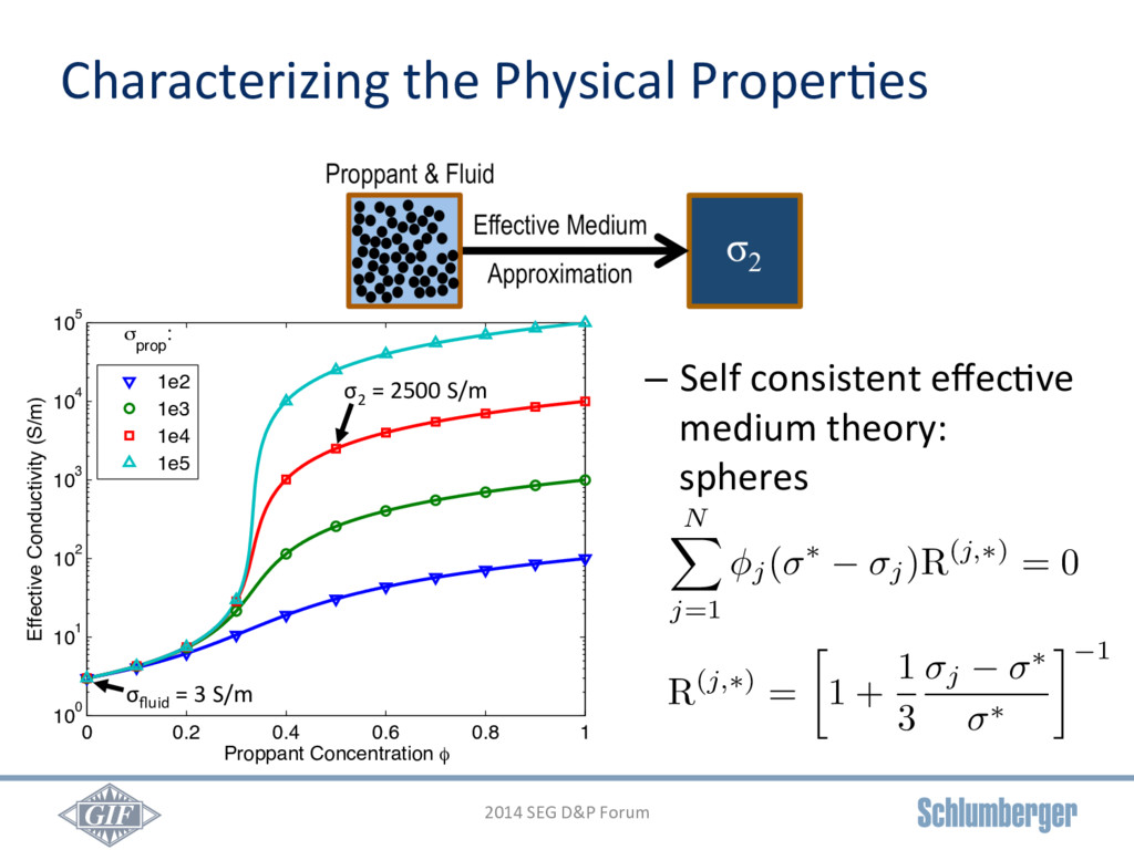
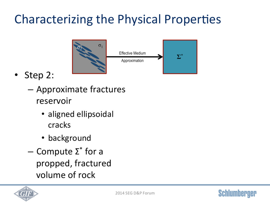
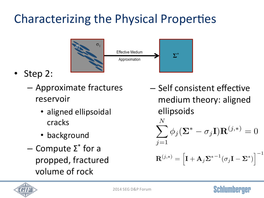
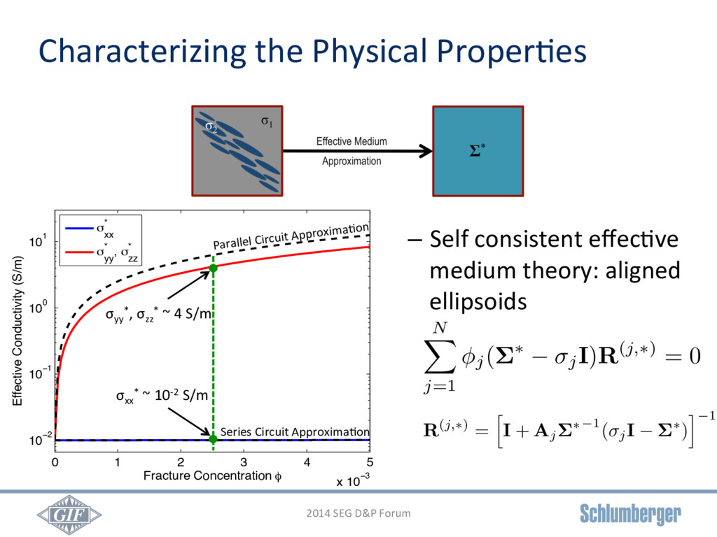
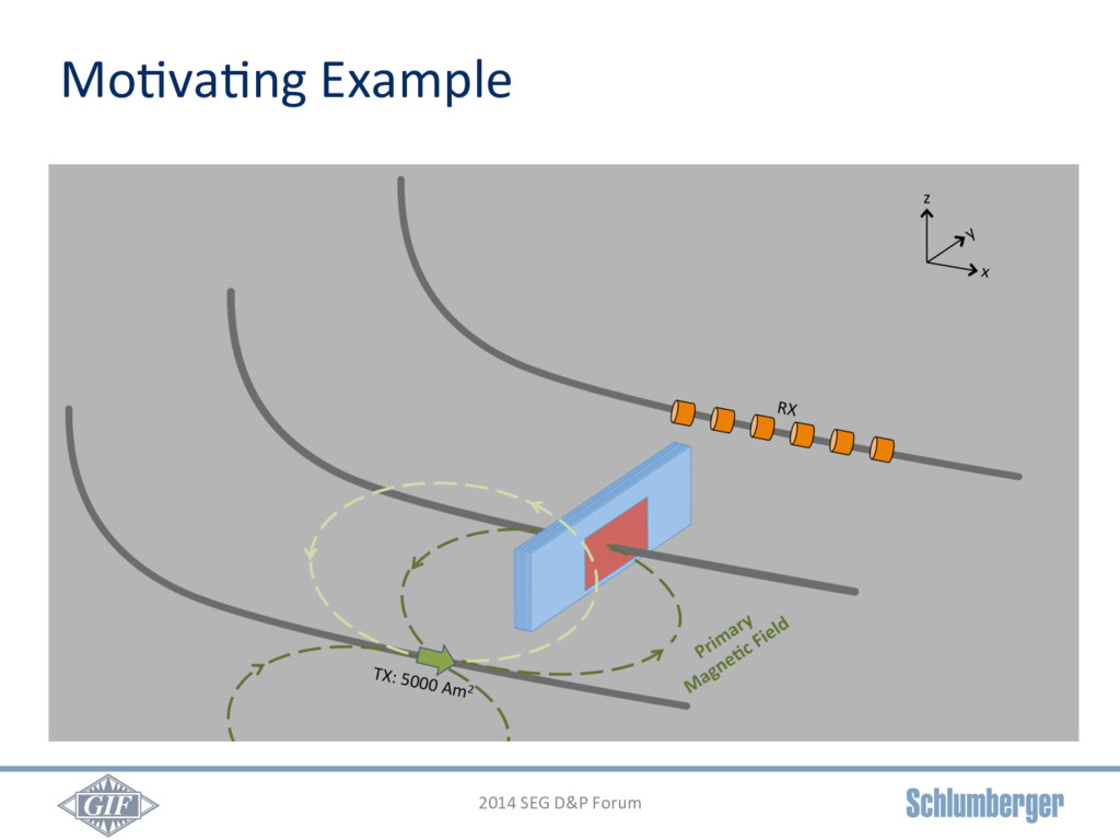
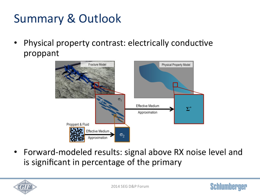
Despite recent advances in hydraulic fracturing and monitoring technologies, there are still many unknowns; chief among them is the extent and distribution of proppant within the reservoir. Here we investigate the potential of introducing highly conductive particles into the proppant and imaging the location of the proppant using electromagnetic surveys. Simulating expected responses, and thus determining if the technique is viable, requires upscaling the physical property structure from a millimeter scale to a meter scale. This upscaling can be completed using analytical or semi-analytical methods such as effective medium theory, or it can be done numerically by formulating upscaling as a parameter estimation problem. Both approaches provide valuable insight into bulk the electromagnetic properties of a doped, fractured reservoir, and the lessons taken from each strengthen our understanding of the electromagnetic characterization of such a reservoir. This understanding is essential for designing a survey capable of detecting the proppant, and once the data have been collected, for approaching the inverse problem.

Transcript

1. GIF The University of Bri0sh Columbia Geophysical Inversion Facility Lindsey J. Heagy*, Douglas W. Oldenburg Geophysical Inversion Facility, University of Bri0sh Columbia lheagy@eos.ubc.ca Collaborators: Michael Wilt, Jiuping Chen Schlumberger EMI Technology Center Using electromagne0cs to delineate proppant distribu0on in a hydraulically fractured reservoir 2014 SEG D&P Forum
2. GIF 2014 SEG D&P Forum •  Used to create pathways for hydrocarbons to flow Hydraulic Fracturing Process Seal off sec0on of wellbore Pump fluid to fracture rock Pump proppant to keep fractures open (Na0onal Energy Board, Canada, 2009)
3. GIF 2014 SEG D&P Forum •  Used to create pathways for hydrocarbons to flow •  Comple0ons parameters: –  well spacing –  stage spacing –  volume of proppant –  volume of fluid –  pumping pressures –  … Hydraulic Fracturing Process (Na0onal Energy Board, Canada, 2009)
4. GIF 2014 SEG D&P Forum •  How do we op0mize fracture comple0ons? Hydraulic Fracturing Process (Na0onal Energy Board, Canada, 2009)
5. GIF Hydraulic Fracturing Process •  How do we op0mize fracture comple0ons? •  Before that… 2014 SEG D&P Forum –  need to understand impact on the reservoir •  fracture geometry •  produc0on / injec0on behavior •  distribu0on of proppant (Na0onal Energy Board, Canada, 2009)
6. GIF Hydraulic Fracturing Process •  How do we op0mize fracture comple0ons? •  Before that… 2014 SEG D&P Forum –  need to understand impact on the reservoir •  fracture geometry •  produc0on / injec0on behavior •  distribu0on of proppant (Na0onal Energy Board, Canada, 2009)
7. GIF Current Fracture Monitoring Techniques •  Far Well: –  Microseismic –  Tiltmeters –  Pressure –  Fiber Op0cs •  Near Well: –  Logs –  Tracers 2014 SEG D&P Forum •  s (Maxwell, 2011)
8. GIF Current Fracture Monitoring Techniques •  Far Well: –  Microseismic –  Tiltmeters –  Pressure –  Fiber Op0cs •  Near Well: –  Logs –  Tracers 2014 SEG D&P Forum (Dusseault and McLennan, 2011)
9. GIF Current Fracture Monitoring Techniques •  Far Well: –  Microseismic –  Tiltmeters –  Pressure –  Fiber Op0cs •  Near Well: –  Logs –  Tracers 2014 SEG D&P Forum Limited sensi0vity to proppant distribu0on (Dusseault and McLennan, 2011)
10. GIF 2014 SEG D&P Forum Imaging the Propped Volume Requirements: 1. Physical property contrast 1. Electrically Conduc0ve Proppant 2. Survey sensi0ve to contrast 2. Electromagne0c Survey 3. Interpret / Invert data
11. GIF 2014 SEG D&P Forum Imaging the Propped Volume Requirements: Approach: 1. Physical property contrast 1. Electrically Conduc0ve Proppant 2. Survey sensi0ve to contrast 2. Electromagne0c Survey 3. Interpret / Invert data
12. GIF Physical Property Model •  What does a fracture look like as an electrical conduc0vity target? •  Scales: –  Proppant: μm-mm –  Fracture geometry •  Length: 100’s m •  Height: 10’s m •  Width: μm-mm 2014 SEG D&P Forum
13. GIF Physical Property Model 2014 SEG D&P Forum
14. GIF 2014 SEG D&P Forum Mo0va0ng Example
15. GIF Mo0va0ng Example •  10 Fractures: –  each 2.5mm wide –  spaced evenly over 10m horizontal segment •  Propped Region: –  70x70m area –  50% proppant –  50% fluid 2014 SEG D&P Forum
16. GIF Characterizing the Physical Proper0es •  Step 1: –  Assume fractures filled with •  conduc0ve proppant •  fluid –  Compute σ2 for a proppant-fluid mixture 2014 SEG D&P Forum
17. GIF Characterizing the Physical Proper0es •  Step 1: –  Assume fractures filled with •  conduc0ve proppant •  fluid –  Compute σ2 for a proppant-fluid mixture –  Self consistent effec0ve medium theory: spheres 2014 SEG D&P Forum R(j,⇤) =  1 + 1 3 j ⇤ ⇤ 1 N X j=1 j( ⇤ j)R(j,⇤) = 0
18. GIF •  Step 1: –  Assume fractures filled with •  conduc0ve proppant •  fluid –  Compute σ2 for a proppant-fluid mixture 2014 SEG D&P Forum 0 0.2 0.4 0.6 0.8 1 100 101 102 103 104 105 Proppant Concentration φ Effective Conductivity (S/m) 1e2 1e3 1e4 1e5 σ prop : σfluid = 3 S/m σ2 = 2500 S/m Characterizing the Physical Proper0es R(j,⇤) =  1 + 1 3 j ⇤ ⇤ 1 N X j=1 j( ⇤ j)R(j,⇤) = 0 –  Self consistent effec0ve medium theory: spheres
19. GIF Characterizing the Physical Proper0es •  Step 2: –  Approximate fractures reservoir •  aligned ellipsoidal cracks •  background –  Compute Σ* for a propped, fractured volume of rock 2014 SEG D&P Forum
20. GIF Characterizing the Physical Proper0es •  Step 2: –  Approximate fractures reservoir •  aligned ellipsoidal cracks •  background –  Compute Σ* for a propped, fractured volume of rock 2014 SEG D&P Forum –  Self consistent effec0ve medium theory: aligned ellipsoids N X j=1 j(⌃⇤ jI)R(j,⇤) = 0 R(j,⇤) = h I + Aj⌃⇤ 1( jI ⌃⇤) i 1
21. GIF Characterizing the Physical Proper0es •  Step 2: –  Approximate fractured volume of rock as •  collec0on of aligned ellipsoidal cracks •  in a background –  Compute Σ* for a propped, fractured volume of rock 2014 SEG D&P Forum 0 1 2 3 4 5 x 10−3 10−2 10−1 100 101 Fracture Concentration φ Effective Conductivity (S/m) σ xx * σ yy * , σ zz * Parallel Circuit Approxima0on Series Circuit Approxima0on σxx * ~ 10-2 S/m σyy *, σzz * ~ 4 S/m –  Self consistent effec0ve medium theory: aligned ellipsoids N X j=1 j(⌃⇤ jI)R(j,⇤) = 0 R(j,⇤) = h I + Aj⌃⇤ 1( jI ⌃⇤) i 1
22. GIF 2014 SEG D&P Forum Mo0va0ng Example
23. GIF 2014 SEG D&P Forum Mo0va0ng Example
24. GIF 2014 SEG D&P Forum Mo0va0ng Example
25. GIF −250 −200 −150 −100 −50 0 50 100 150 200 250 −5 0 5 10 15 RX position (m) Magnetic Flux (pT) Measured B x 200Hz 500Hz 1000Hz −250 −200 −150 −100 −50 0 50 100 150 200 250 −0.4 −0.3 −0.2 −0.1 0 0.1 RX position (m) Magnetic Flux (pT) Secondary B x 200Hz 500Hz 1000Hz −250 −200 −150 −100 −50 0 50 100 150 200 250 −10 −5 0 5 RX position (m) Magnetic Flux (%) Secondary B x 200Hz 500Hz 1000Hz Magne0c Responses •  Measurements: –  TX Frequency Range: 10Hz to 2kHz –  In-phase and quadrature –  3 spa0al components: x,y,z •  To detect fracture: –  Signal & Secondary above RX noise floor •  10-2 pT –  Secondary a sufficient percentage of primary RX Noise Floor: 10-2 pT RX Noise Floor: 10-2 pT 1% Cut-off In-Phase, Bx component Frac No Frac
26. GIF 2014 SEG D&P Forum TX Position (m) RX Position (m) −200 0 200 −200 −100 0 100 200 Magnetic Flux (pT) −0.3 −0.25 −0.2 −0.15 −0.1 −0.05 TX Position (m) RX Position (m) −200 0 200 −200 −100 0 100 200 Magnetic Flux (%) −8 −6 −4 −2 •  Measurements: –  TX Frequency Range: 10Hz to 2kHz –  In-phase and quadrature –  3 spa0al components: x,y,z •  To detect fracture: –  Signal & Secondary above RX noise floor •  10-2 pT –  Secondary a sufficient percentage of primary Magne0c Responses In-Phase, Bx component 1000 Hz
27. GIF 2014 SEG D&P Forum •  Physical property contrast: electrically conduc0ve proppant •  Forward-modeled results: signal above RX noise level and is significant in percentage of the primary Summary & Outlook
28. GIF Summary & Outlook •  Moving forward: –  increase complexity of models –  examine the survey design –  invert the 3D electromagne0c data 2014 SEG D&P Forum 1. Electrically Conduc0ve Proppant 2. Electromagne0c Survey 3. Interpret / Invert data Goal: to ascertain under what condi0ons EM imaging can provide cost effec0ve informa0on about proppant distribu0on in a fractured reservoir.
29. GIF 2014 SEG D&P Forum •  Thanks to Nestor Cuevas and Ping Zhang for their contribu0ons to this project •  Thanks to Christoph Schwarzbach for the forward modeling code Acknowledgements
30. GIF 2014 SEG D&P Forum Ques0ons? Thank you!
31. GIF 2014 SEG D&P Forum •  Berryman, J. G. & Hoversten, G. M. Modelling electrical conduc0vity for earth media with macroscopic fluid-filled fractures. Geophys. Prospect. 61, 471–493 (2013). •  Bruggeman, D. A. G. The calcula0on of various physical constants of heterogeneous substances. I. The dielectric constants and conduc0vi0es of mixtures composed of isotropic substances. Ann. Phys. 416, 636–664 (1935). •  Cipolla, C. L., Warpinski, N. R., Mayerhofer, M. J. & Technologies, P. SPE 115771 Hydraulic Fracture Complexity : Diagnosis , Remedia0on , and Exploita0on. 20–22 (2008). •  Dusseault, M., & McLennan, J. (2011). Massive mul0-stage hydraulic fracturing: Where are we?. ARMA (American Rock Mechanics Associa7on) e-Newsle=er. Published, 1, 2011. •  Maxwell, S.C., Hydraulic fracture height growth. Recorder 36, 18-22 (2011) •  Shafiro, B. & Kachanov, M. Anisotropic effec0ve conduc0vity of materials with nonrandomly oriented inclusions of diverse ellipsoidal shapes. J. Appl. Phys. 87, 8561–8569 (2000). •  Torquato, S. Random Heterogeneous Materials: Microstructure and Macroscopic Proper7es. (Springer, 2002). •  Wilt, M. J. et al. Crosswell electromagne0c tomography: System design considera0ons and field results. Geophysics 60, 871–885 (1995). •  hzp://www.neb-one.gc.ca/clf-nsi/archives/rnrgynfmtn/nrgyrprt/ntrlgs/prmrndrstndngshlgs2009/ prmrndrstndngshlgs2009-eng.html References
32. GIF 2014 SEG D&P Forum Fracture Geometries (Cipolla, 2008)
33. GIF 2014 SEG D&P Forum Fracture Geometries (Cipolla, 2008)
34. GIF 2014 SEG D&P Forum Mo0va0ng Example
35. GIF −250 −200 −150 −100 −50 0 50 100 150 200 250 −0.2 0 0.2 0.4 0.6 RX position (m) Magnetic Flux (pT) Measured B x 200Hz 500Hz 1000Hz −250 −200 −150 −100 −50 0 50 100 150 200 250 −0.6 −0.4 −0.2 0 0.2 RX position (m) Magnetic Flux (pT) Secondary B x 200Hz 500Hz 1000Hz −250 −200 −150 −100 −50 0 50 100 150 200 250 −150 −100 −50 0 50 RX position (m) Magnetic Flux (%) Secondary B x 200Hz 500Hz 1000Hz Magne0c Responses •  Measurements: –  TX Frequency Range: 10Hz to 2kHz –  In-phase and quadrature –  3 spa0al components: x,y,z •  To detect fracture: –  Signal & Secondary above RX noise floor •  10-2 pT –  Secondary a sufficient percentage of primary RX Noise Floor: 10-2 pT RX Noise Floor: 10-2 pT 1% Cut-off In-Phase, Bx component Fracture Primary
36. GIF TX Position (m) RX Position (m) −200 0 200 −200 −100 0 100 200 Magnetic Flux (pT) −0.4 −0.3 −0.2 −0.1 TX Position (m) RX Position (m) −200 0 200 −200 −100 0 100 200 Magnetic Flux (%) −100 −80 −60 −40 −20 2014 SEG D&P Forum •  Measurements: –  TX Frequency Range: 10Hz to 2kHz –  In-phase and quadrature –  3 spa0al components: x,y,z •  To detect fracture: –  Signal & Secondary above RX noise floor •  10-2 pT –  Secondary a sufficient percentage of primary Magne0c Responses In-Phase, Bx component 1000 Hz
37. GIF Single Inclusion Solu0ons •  Inside a sphere •  Inside an Ellipsoid 2014 SEG D&P Forum E = R(2,1)E0 R(2,1) =  1 + 1 3 2 1 1 1 E = e R(2,1)E0 e R(2,1) =  e I + e A2 2 1 1 1
38. GIF Maxwell Approxima0on •  Spherical Inclusions •  Ellipsoidal Inclusions 2014 SEG D&P Forum R(j,1) =  1 + 1 3 j 1 1 1 N X j=1 j( ⇤ j)R(j,1) = 0 e R(j,1) =  e I + e Aj j 1 1 1 N X j=1 j(e ⌃⇤ j e I)e R(j,1) = 0
39. GIF Self Consistent Approxima0on 2014 SEG D&P Forum e R(j,⇤) = h e I + e Aj e ⌃⇤ 1 ( j e I e ⌃⇤) i 1 N X j=1 j(e ⌃⇤ j e I)e R(j,⇤) = 0 R(j,⇤) =  1 + 1 3 j ⇤ ⇤ 1 N X j=1 j( ⇤ j)R(j,⇤) = 0 Spherical Inclusions Ellipsoidal Inclusions
40. GIF Self Consistent Approxima0on 2014 SEG D&P Forum e R(j,⇤) = h e I + e Aj e ⌃⇤ 1 ( j e I e ⌃⇤) i 1 N X j=1 j(e ⌃⇤ j e I)e R(j,⇤) = 0 R(j,⇤) =  1 + 1 3 j ⇤ ⇤ 1 N X j=1 j( ⇤ j)R(j,⇤) = 0 Spherical Inclusions Ellipsoidal Inclusions