fmm3dbie-devel-pres

Locally corrected quadratures scheme and data structures presentation

Transcript

1. fmm3dbie - devel fmm3dbie - a library for • fmm-accelerated layer potential evaluators • Iterative solvers using them • robust locally corrected quadrature methods • matrix entry generator for fast direct solvers • Ability to interface with varied CAD formats • Interfaces in Fortran/C/Python/MATLAB(?) (Δ + k2)u = 0 in Ω u = g on ∂Ω = Γ u = αSk [σ] + βDk [σ] g = − βσ/2 + αSk [σ] + βDk [σ]
2. Surface representation • ! • Chart for ! • Supported elements ! : • ! , basis on ! , where ! are Koornwinder polynomials, and discretization nodes Vioreanu- Rokhlin nodes Γ = ∪j Γj Γj = xj, i.e., xj : B → Γj B T0 = {(u, v) : u > 0, v > 0, u + v < 1} T0 = {Knm (u, v), n + m < p} Knm Γj xj
3. Near-far quadrature split Rj cj Γ j ηR j N η (Γ j ) • Centroid: ! • Bounding sphere radius ! • ! -scaled near-field of ! : ! • ! : collection of patches for which ! is in the near-field — dual of ! ! cj = ∫ Γj xda Rj = min R {R : Γj ⊂ BR (cj )} η Γj Nη (Γj ) = {x : |x − cj | ≤ ηRj } Tη (x) x Nη (Γj ) Tη (x) = {Γj : x ∈ Nη (Γj )} = {Γj : |x − cj | ≤ ηRj } S[σ](x) = ∑ j ∫ Γj G(x, y)σ(y)da(y) = ∑ Γj ∈Tη (x) ∫ Γj G(x, y)σ(y)da(y) + ∑ Γj ∉Tη (x) ∫ Γj G(x, y)σ(y)da(y) = Snear [σ](x) + Sfar [σ](x) Precomputed in a target dependent manner Target independent oversampled quadrature
4. Near quadrature Instead compute: ! bj ℓ (x) = ∫ B G(x, xj)Pℓ (u, v)Jj(u, v) dudv ℓ = 1,…nb ∫ Γj G(x, y)σ(y)da(y) = ∫ B G(x, xj(u, v))σ(u, v)Jj(u, v)dudv Jj(u, v) = |∂u xj × ∂v xj | Suppose orthogonal polynomials on Pj (u, v) : B , denote the samples of the density on patch σj ℓ ℓ = 1,2,…nb Γj Find such that: aj ℓ (x) nb ∑ j=1 aj ℓ (x)σj ℓ − ∫ B G(x, xj(u, v))σ(u, v)Jj(u, v) dudv < ε aj 1:nb = U ⋅ bj 1:nb is the coefficients to values matrix U ∈ ℝnb ×nb
5. Near quadrature - optimizations • Oversampled quadrature for ! — avoids branching and can use BLAS routines for better performance. No need to suffer for high oversampling for all targets • Request lower precision for adaptive integration for targets in ! Nη (Γj )∖Nη1 (Γj ) Nη1 (Γj )
6. Far quadrature - oversampling estimation • Identify 10 furthest targets in ! (If ! , then choose ! targets from the list • Add 15 (or 25 - ! if ! ) randomly chosen targets on ! • Let ! denote the union of these two sets of targets • Depending on the order (o) of the kernel (order = -1 for ! , 0 for ! , 1 for ! and so on), consider the integrals ! • Let ! denote approximations to ! computed using order ! nodes on ! • Then ! for patch ! is given by Nη (Γj ) |Nη (Γj )| < 20 |Nη (Γj )|/2 |Nη (Γj )|/2 |Nη (Γj )| < 20 ∂BηRj (cj ) F(Γj ) S D S′′ Iℓ [x] = ∫ B ∂(o+1) n G(x, xj(u, v))Pℓ (u, v)Jj(u, v)dudv Iℓ,q [x] Iℓ [x] q B qj Γj qj = min q max 0 ≤ ℓ < nb x ∈ F(Γj ) |Iℓ,q [x] − Iℓ,q+1 [x]| < ε
7. Choice of η p ÷ 1.25 2.00 2.75 2 24.1 7.45 5 3 10.6 4.67 3.26 4 8.76 2.8 2.8 6 3.92 2.14 1.4 8 2.39 1.25 1.25 (a) m p ÷ 1.25 2.00 2.75 2 23.6 65.6 137 3 50.4 134 276 4 82.3 222 458 6 173 466 961 8 298 798 1650 (b) – p ÷ 1.25 2.00 2.75 2 6050 5280 4050 3 4820 3980 3240 4 3730 3490 2710 6 2070 1820 1590 8 1310 1180 956 (c) SNEAR p ÷ 1.25 2.00 2.75 2 1200 2870 3790 3 2180 3440 3670 4 2210 4080 3460 6 3230 4270 3860 8 3740 4660 3500 (d) SLP Table 1: m,–,SNEAR, and SLP as a function of p and ÷ {tab:numerical-e • ! , if ! • ! , if ! • ! , if ! η = 1.25 p > 8 η = 2 4 < p ≤ 8 η = 2.75 p ≤ 4 • ! : effective memory required per discretization node • ! • ! : speed of quadrature generation in pts/sec/core • ! : speed of layer potential evaluation in pts/sec/core α m = Nover /N Snear SLP
8. Performance results p Á 5 · 10≠3 5 · 10≠4 5 · 10≠7 5 · 10≠10 2 1 1.62 5 9.58 3 0.701 1 3.26 7.15 4 0.6 1.03 2.8 4.77 6 0.714 0.87 2.14 3.15 8 0.778 1.17 2.39 2.53 (a) m p Á 5 · 10≠3 5 · 10≠4 5 · 10≠7 5 · 10≠10 2 137 137 137 137 3 276 276 276 276 4 222 222 222 222 6 466 466 466 466 8 298 298 298 298 (b) – p Á 5 · 10≠3 5 · 10≠4 5 · 10≠7 5 · 10≠10 2 10900 8800 4230 1290 3 7850 7810 3340 1170 4 8270 8410 3270 938 6 3260 3280 1810 773 8 2150 2100 1330 636 (c) SNEAR p Á 5 · 10≠3 5 · 10≠4 5 · 10≠7 5 · 10≠10 2 14000 10200 3710 1230 3 12900 10300 3670 1380 4 13300 10800 4110 2040 6 11600 10200 4160 2400 8 11400 8930 3730 2800 (d) SLP Table 2: m,–,s1, and s2 as a function of p and Á {tab:numerical-perf-res} aavg 1.61 2.33 4.66 9.31 14 Npatches 2400 2304 2450 2304 2400 m 2.8 2.8 2.8 2.8 2.8 – 222 305 603 1240 1870 SNEAR 3610 2730 1560 780 499 S 4110 3880 3180 2330 1650 • ! : effective memory required per discretization node • ! • ! : speed of quadrature generation in pts/sec/core • ! : speed of layer potential evaluation in pts/sec/core α m = Nover /N Snear SLP
9. Order of convergence Figure 6: Left: Relative L2 error in green’s identity Ág Right: relative LŒ error in solution to integral equation Áa . In both figures, the dashed colored lines are reference curves for hp≠1 for the corresponding p. The dashed black line is a reference line for Á {f where u is a solution to Helmholtz equation in the interior of the region generated by a point source located in the exterior of the domain. The second test is to solve a combined field integral equation for the unknown density ‡
10. Big example
11. Ways to get involved • Request features at developer meetings • Develop existing feature requests on the repo • Wrappers for other PDEs and representations • Maxwell: MFIE + CFIE + EFIE wrappers (#4) • Maxwell: NRCCIE (#7) • Maxwell: CSIE (#8) • Stokes : Combined field rep for velocity BVP (#9) • Stokes: Single layer for traction problem (#10) • Stokes: Mobility problem, combined field representation (#11) • Stokes: Mobility adjoint representation with single layer (#12) • Openmp optimizations for base routines • Cumulative sum (#2) • Convert (i,j) pairs to column sparse compressed format (#5) • Incorporate new quadrature schemes • Local QBX (#13) • Hedgehog (#14) • Incorporate new types of patches (! , associated discretization nodes, orthogonal polynomials) • Triangle ! with Gmsh nodes (#15) • I/O • Read in .msh files (#16) • Vtk files for plotting vector fields (#17) List of open tasks Developer process B T0
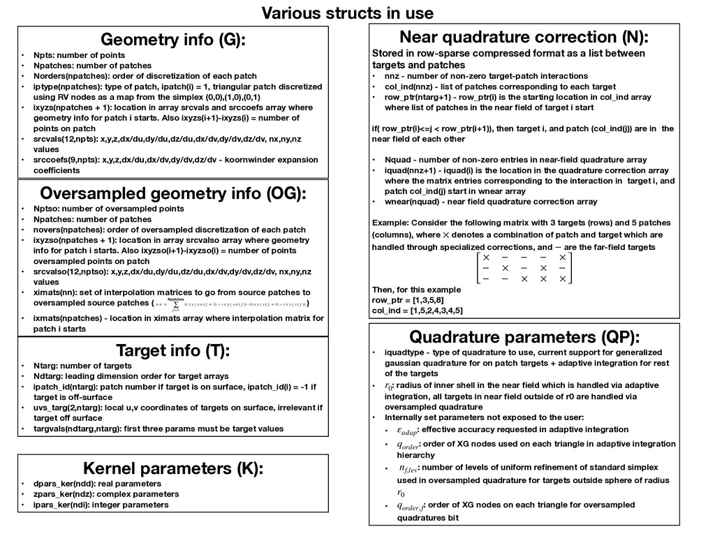
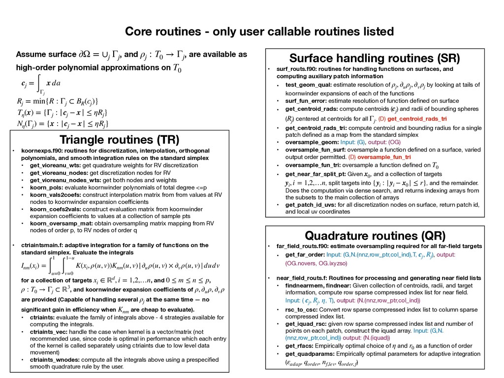
12. Geometry info (G): • Npts: number of points • Npatches: number of patches • Norders(npatches): order of discretization of each patch • iptype(npatches): type of patch, ipatch(i) = 1, triangular patch discretized using RV nodes as a map from the simplex (0,0),(1,0),(0,1) • ixyzs(npatches + 1): location in array srcvals and srccoefs array where geometry info for patch i starts. Also ixyzs(i+1)-ixyzs(i) = number of points on patch • srcvals(12,npts): x,y,z,dx/du,dy/du,dz/du,dx/dv,dy/dv,dz/dv, nx,ny,nz values • srccoefs(9,npts): x,y,z,dx/du,dx/dv,dy/dv,dz/dv - koornwinder expansion coefficients Oversampled geometry info (OG): • Nptso: number of oversampled points • Npatches: number of patches • novers(npatches): order of oversampled discretization of each patch • ixyzso(npatches + 1): location in array srcvalso array where geometry info for patch i starts. Also ixyzso(i+1)-ixyzso(i) = number of points oversampled points on patch • srcvalso(12,nptso): x,y,z,dx/du,dy/du,dz/du,dx/dv,dy/dv,dz/dv, nx,ny,nz values • ximats(nn): set of interpolation matrices to go from source patches to oversampled source patches ( ) • ixmats(npatches) - location in ximats array where interpolation matrix for patch i starts n n = Npatches ∑ j=1 (i x y z s o ( j + 1) − i x y z s o ( j )) ⋅ (i x y z s ( j + 1) − i x y z s ( j )) Target info (T): • Ntarg: number of targets • Ndtarg: leading dimension order for target arrays • ipatch_id(ntarg): patch number if target is on surface, ipatch_id(i) = -1 if target is off-surface • uvs_targ(2,ntarg): local u,v coordinates of targets on surface, irrelevant if target off surface • targvals(ndtarg,ntarg): first three params must be target values Near quadrature correction (N): Stored in row-sparse compressed format as a list between targets and patches • nnz - number of non-zero target-patch interactions • col_ind(nnz) - list of patches corresponding to each target • row_ptr(ntarg+1) - row_ptr(i) is the starting location in col_ind array where list of patches in the near field of target i start if( row_ptr(i)<=j < row_ptr(i+1)), then target i, and patch (col_ind(j)) are in the near field of each other • Nquad - number of non-zero entries in near-field quadrature array • iquad(nnz+1) - iquad(i) is the location in the quadrature correction array where the matrix entries corresponding to the interaction in target i, and patch col_ind(j) start in wnear array • wnear(nquad) - near field quadrature correction array Example: Consider the following matrix with 3 targets (rows) and 5 patches (columns), where denotes a combination of patch and target which are handled through specialized corrections, and are the far-field targets Then, for this example row_ptr = [1,3,5,8] col_ind = [1,5,2,4,3,4,5] × − [ × − − − × − × − × − − − × × × ] Kernel parameters (K): • dpars_ker(ndd): real parameters • zpars_ker(ndz): complex parameters • ipars_ker(ndi): integer parameters Quadrature parameters (QP): • iquadtype - type of quadrature to use, current support for generalized gaussian quadrature for on patch targets + adaptive integration for rest of the targets • : radius of inner shell in the near field which is handled via adaptive integration, all targets in near field outside of r0 are handled via oversampled quadrature • Internally set parameters not exposed to the user: • : effective accuracy requested in adaptive integration • : order of XG nodes used on each triangle in adaptive integration hierarchy • : number of levels of uniform refinement of standard simplex used in oversampled quadrature for targets outside sphere of radius • : order of XG nodes on each triangle for oversampled quadratures bit r0 εadap qorder nf,lev r0 qorder, f Various structs in use
13. Triangle routines (TR) • koornexps.f90: routines for discretization, interpolation, orthogonal polynomials, and smooth integration rules on the standard simplex • get_vioreanu_wts: get quadrature weights for RV discretization • get_vioreanu_nodes: get discretization nodes for RV • get_vioreanu_nodes_wts: get both nodes and weights • koorn_pols: evaluate koornwinder polynomials of total degree <=p • koorn_vals2coefs: construct interpolation matrix from from values at RV nodes to koornwinder expansion coefficients • koorn_coefs2vals: construct evaluation matrix from koornwinder expansion coefficients to values at a collection of sample pts • koorn_oversamp_mat: obtain oversampling matrix mapping from RV nodes of order p, to RV nodes of order q • ctriaintsmain.f: adaptive integration for a family of functions on the standard simplex. Evaluate the integrals for a collection of targets , and , , and koornwinder expansion coefficients of are provided (Capable of handling several at the same time — no significant gain in efficiency when are cheap to evaluate). • ctriaints: evaluate the family of integrals above - 4 strategies available for computing the integrals. • ctriaints_vec: handle the case when kernel is a vector/matrix (not recommended use, since code is optimal in performance which each entry of the kernel is called separately using ctriaints due to low level data movement) • ctriaints_wnodes: compute all the integrals above using a prespecified smooth quadrature rule by the user. Inm (xi ) = ∫ 1 u=0 ∫ 1−u v=0 K(xi , ρ(u, v))Knm (u, v)|∂u ρ(u, v) × ∂v ρ(u, v)|dudv xi ∈ ℝd, i = 1,2,…n 0 ≤ m ≤ n ≤ p ρ : T0 → Γj ⊂ ℝ3 ρ, ∂u ρ, ∂v ρ ρj Knm Core routines - only user callable routines listed Surface handling routines (SR) • surf_routs.f90: routines for handling functions on surfaces, and computing auxiliary patch information • test_geom_qual: estimate resolution of by looking at tails of koornwinder expansions of each of the functions • surf_fun_error: estimate resolution of function defined on surface • get_centroid_rads: compute centroids ( ) and radii of bounding spheres ( ) centered at centroids for all . (D) get_centroid_rads_tri • get_centroid_rads_tri: compute centroid and bounding radius for a single patch defined as a map from the standard simplex • oversample_geom: Input: (G), output: (OG) • oversample_fun_surf: oversample a function defined on a surface, varied output order permitted. (D) oversample_fun_tri • oversample_fun_tri: oversample a function defined on • get_near_far_split_pt: Given , and a collection of targets , split targets into , and the remainder. Does the computation via dense search, and returns indexing arrays from the subsets to the main collection of arrays • get_patch_id_uvs: for all discretization nodes on surface, return patch id, and local uv coordinates ρj , ∂u ρj , ∂v ρj cj Rj Γj T0 x0 yi , i = 1,2,…n {yi : |yi − x0 | ≤ r} Assume surface , and , are available as high-order polynomial approximations on ∂Ω = ∪j Γj ρj : T0 → Γj T0 cj = ∫ Γj x da Rj = min{R : Γj ⊂ BR (cj )} Quadrature routines (QR) • far_field_routs.f90: estimate oversampling required for all far-field targets • get_far_order: Input: (G,N.(nnz,row_ptr,col_ind),T, ), output: (OG.novers, OG.ixyzso) • near_field_routs.f: Routines for processing and generating near field lists • findnearmem, findnear: Given collection of centroids, radii, and target information, compute row sparse compressed index list for near field. Input: ( , , T), output: (N.(nnz,row_ptr,col_ind)) • rsc_to_csc: Convert row sparse compressed index list to column sparse compressed index list. • get_iquad_rsc: given row sparse compressed index list and number of points on each patch, construct the iquad array. Input: (G,N. (nnz,row_ptr,col_ind)) output: (N.(iquad)) • get_rfacs: Empirically optimal choice of and as a function of order • get_quadparams: Empirically optimal parameters for adaptive integration ( , , , ) cj , Rj cj , Rj η η r0 εadap qorder nf,lev qorder, f Tη (x) = {Γj : |cj − x| ≤ ηRj } Nη (Γj ) = {x : |cj − x| ≤ ηRj }
14. GGQ routines (GGQ) • ggq-quads.f: Generate locally corrected quadrature for scalar kernel • getnearquad_compact_guru: for order -1 operators • getnearquad_pv_guru: for order 0 operators (identity term in limit not included) • Input: (G,N,T,K) output: (N.(wnear)) • (D) SR.get_centroid_rads -> Evaluate • (D) QR.rsc_to_csc: adaptive integration performance is more efficient when all targets for a particular patch are collected. So need to parallelize over source patches, hence need column sparse compressed representation • (D) QR.get_quadparams_adap: Split targets into adaptive integration list and oversampled quadrature processing list • (D) TR.ctriaints: handle adaptive integration targets • (D) TR.ctriaints_wnodes: handle oversampled quadrature targets • (D) Other internal dependencies: get_ggq_self_quad_compact/pv_pt, to evaluate the integrals on self cj , Rj Build your own locally corrected quadrature example - GGQ + adaptive integration
15. Helmholtz combined field wrapper routines - Iterative solvers PDE: (Δ + k2)u = 0 x ∈ Ω u = f x ∈ ∂Ω Representation: u = αk [σ] + βk [σ] BIE: (− β 2 + αk + βPV k ) σ = f Kernel parameters (K): • dpars_ker: N/A • zpars_ker(3): zpars(1) = k, zpars(2) = , zpars(3) = • ipars_ker: N/A α β Iterative solver routines • helm_comb_dir.f: Generate locally corrected quadrature for Helmholtz kernel, apply layer potential, matrix vector application, iterative solver routines, fast direct solver routines • getnearquad_helm_comb_dir: generate near field quadrature correction • Input: (G,N,T,K) output: (N.(wnear)) • (D) GGQ.getnearquad_compact/pv_guru (compact if , pv otherwise) • lpcomp_helm_comb_dir_addsub: layer potential evaluation given near field quadrature correction (computes layer potential for point FMM, then subtracts near contribution, and adds back near correction) ,acts on the oversampled geometry on input, but is oversampled inside the routine (need access to original for applying near quadrature correction) • Input: (OG, N,T,K, ) output: ( interpreted as PV if target on boundary) • (D) Helmholtz FMM • lpcomp_helm_comb_dir_setsub: layer potential evaluation given near field quadrature correction (computes layer potential for point FMM with nearest neighbors (list 1) turned off, then adds near correction, removes near correction which outside of list1, and adds list1 which was not in near correction) ,acts on the oversampled geometry on input, but is oversampled inside the routine (need access to original for applying near quadrature correction) • Input: (OG, N,T,K, ) output: ( interpreted as PV if target on boundary) • (D) SR.oversample_fun_surf • (D) Helmholtz FMM • lpcomp_helm_comb_dir: Simpler calling interface for interface above • Input: (G,T,K, ) output: ( interpreted as PV if target on boundary) • (D) SR.get_centroid_rads • (D) QR.findnearmem, findnear • (D) getnearquad_helm_comb_dir • (D) QR.get_far_order • (D) SR.oversample_geom • (D) lpcomp_helm_comb_dir_addsub β = 0 σ σ σ αk [σ] + βk [σ] σ σ σ αk [σ] + βk [σ] σ αk [σ] + βk [σ] Iterative solver routines (2) • helm_comb_dir.f: Generate locally corrected quadrature for Helmholtz kernel, apply layer potential, matrix vector application, iterative solver routines, fast direct solver routines • helm_comb_dir_solver: Simpler calling interface for interface above • Input: (G,T,K, ) output: ( interpreted as PV if target on boundary) • (D) SR.get_centroid_rads • (D) QR.findnearmem, findnear • (D) getnearquad_helm_comb_dir • (D) QR.get_far_order • (D) SR.oversample_geom σ αk [σ] + βk [σ]