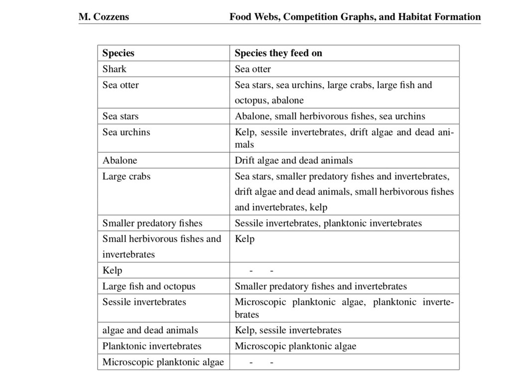
('sea otter', 'sea urchins'), ('sea otter', 'large crabs'), ('sea otter', 'large fish and octopus'), ('sea otter', 'abalone'), ('sea stars', 'abalone'), ('sea stars', 'small herbivorous fishes'), ('sea stars', 'sea urchins'), ('sea urchins', 'kelp'), ('sea urchins', 'sessile invertebrates'), ('sea urchins', 'algae'), ('large crabs', 'sea stars'), ('large crabs', 'smaller predatory fishes'), ('large crabs', 'algae'), ('large crabs', 'small herbivorous fishes'), ('large crabs', 'kelp'), ('large fish and octopus', 'smaller predatory fishes'), ('abalone', 'algae'), ('small herbivorous fishes', 'kelp'), ('sessile invertebrates', 'microscopic planktonic algae'), ('sessile invertebrates', 'planktonic invertebrates'), ('algae', 'kelp'), ('algae', 'sessile invertebrates'), ('smaller predatory fishes', 'sessile invertebrates'), ('smaller predatory fishes', 'planktonic invertebrates'), ('planktonic invertebrates', 'microscopic planktonic algae')]
![In [1]: # !pip install camelot-py[cv] import pandas as pd](https://files.speakerdeck.com/presentations/35e5cc917e8940cc996e0143fa307bbe/slide_11.jpg)
![In [2]: print('>', len(tables)) df = tables[0].df df Out[2]: 0](https://files.speakerdeck.com/presentations/35e5cc917e8940cc996e0143fa307bbe/slide_12.jpg)
![In [3]: df.columns = ['pred', 'prey'] df = df.reindex(df.index.drop(0)) mapping](https://files.speakerdeck.com/presentations/35e5cc917e8940cc996e0143fa307bbe/slide_13.jpg)
![In [4]: import re print(mapping['microscopicplanktonicalgae']) def fix_text(text, mapping): for k,](https://files.speakerdeck.com/presentations/35e5cc917e8940cc996e0143fa307bbe/slide_14.jpg)
![In [7]: df.head() Out[7]: pred prey 1 shark sea otter](https://files.speakerdeck.com/presentations/35e5cc917e8940cc996e0143fa307bbe/slide_15.jpg)
![In [8]: ( df.prey .str .split(',', expand=True) .stack() .reset_index(drop=True, level=1)](https://files.speakerdeck.com/presentations/35e5cc917e8940cc996e0143fa307bbe/slide_16.jpg)
![In [9]: df = df.drop('prey', axis=1).join( df.prey .str .split(',', expand=True)](https://files.speakerdeck.com/presentations/35e5cc917e8940cc996e0143fa307bbe/slide_17.jpg)
![In [10]: df = df[df['prey'] != '--'] df.loc[:,'prey'] = df['prey'].str.strip()](https://files.speakerdeck.com/presentations/35e5cc917e8940cc996e0143fa307bbe/slide_18.jpg)
![In [12]: df.to_csv('data/food_web.csv', index=False) df.head() Out[12]: pred prey 0 shark](https://files.speakerdeck.com/presentations/35e5cc917e8940cc996e0143fa307bbe/slide_19.jpg)
![In [13]: In [14]: import numpy as np import networkx](https://files.speakerdeck.com/presentations/35e5cc917e8940cc996e0143fa307bbe/slide_20.jpg)
![In [15]: df = pd.read_csv('data/food_web.csv') G = nx.from_pandas_edgelist( df, source='pred',](https://files.speakerdeck.com/presentations/35e5cc917e8940cc996e0143fa307bbe/slide_21.jpg)
![In [16]: from pprint import pprint pprint(list(G.nodes)) ['shark', 'sea otter',](https://files.speakerdeck.com/presentations/35e5cc917e8940cc996e0143fa307bbe/slide_22.jpg)
![In [17]: pprint(list(G.edges)) [('shark', 'sea otter'), ('sea otter', 'sea stars'),](https://files.speakerdeck.com/presentations/35e5cc917e8940cc996e0143fa307bbe/slide_23.jpg)
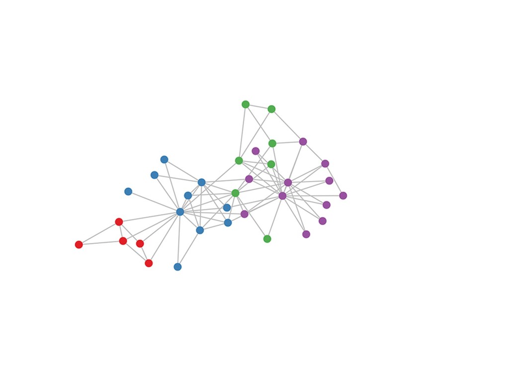
![In [18]: np.random.seed(1) plt.figure(figsize=(10, 8)) nx.draw_networkx(G, node_color='green') plt.xticks([]) plt.yticks([]);](https://files.speakerdeck.com/presentations/35e5cc917e8940cc996e0143fa307bbe/slide_24.jpg)
![In [19]: def pagerank(G, alpha=0.85, max_iter=100, tol=1.0e-6): W = nx.stochastic_graph(G)](https://files.speakerdeck.com/presentations/35e5cc917e8940cc996e0143fa307bbe/slide_26.jpg)
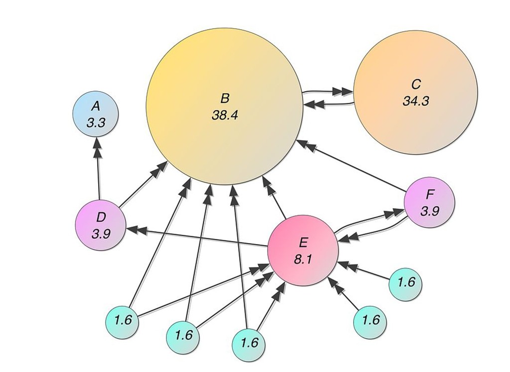
![In [20]: In [21]: pprint(pagerank(G, alpha=0.85)) pprint(nx.pagerank(G, alpha=0.85)) {'abalone': 0.04940106801052845,](https://files.speakerdeck.com/presentations/35e5cc917e8940cc996e0143fa307bbe/slide_27.jpg)
![In [22]: In [23]: pageranks = pagerank(G, alpha=0.85) for g](https://files.speakerdeck.com/presentations/35e5cc917e8940cc996e0143fa307bbe/slide_28.jpg)
![In [24]: import altair as alt import nx_altair as nxa](https://files.speakerdeck.com/presentations/35e5cc917e8940cc996e0143fa307bbe/slide_29.jpg)
![In [25]: pr_viz.interactive().properties(width=500, height=400) Out[25]:](https://files.speakerdeck.com/presentations/35e5cc917e8940cc996e0143fa307bbe/slide_30.jpg)
![In [26]: in_degree = dict(G.in_degree) pprint(in_degree) {'abalone': 2, 'algae': 3,](https://files.speakerdeck.com/presentations/35e5cc917e8940cc996e0143fa307bbe/slide_32.jpg)
![In [27]: for g in G.nodes(): G.nodes[g]['name'] = g G.nodes[g]['in_degree']](https://files.speakerdeck.com/presentations/35e5cc917e8940cc996e0143fa307bbe/slide_33.jpg)
![In [28]: hub_viz.interactive().properties(width=500, height=400) Out[28]:](https://files.speakerdeck.com/presentations/35e5cc917e8940cc996e0143fa307bbe/slide_34.jpg)
![In [29]: import pandas as pd CATEGORIES = [ 'goals',](https://files.speakerdeck.com/presentations/35e5cc917e8940cc996e0143fa307bbe/slide_43.jpg)
![In [30]: import numpy as np np.random.seed(1) df.sample(10) Out[30]: name](https://files.speakerdeck.com/presentations/35e5cc917e8940cc996e0143fa307bbe/slide_44.jpg)
![In [31]: from sklearn.model_selection import train_test_split target = 'adp' y](https://files.speakerdeck.com/presentations/35e5cc917e8940cc996e0143fa307bbe/slide_45.jpg)
![In [32]: from sklearn.preprocessing import LabelBinarizer, StandardScaler from sklearn_pandas import](https://files.speakerdeck.com/presentations/35e5cc917e8940cc996e0143fa307bbe/slide_46.jpg)
![In [33]: ♀ ♀ from sklearn.linear_model import LinearRegression lr =](https://files.speakerdeck.com/presentations/35e5cc917e8940cc996e0143fa307bbe/slide_47.jpg)
![In [34]: #!pip install mord import mord model = mord.OrdinalRidge(fit_intercept=False)](https://files.speakerdeck.com/presentations/35e5cc917e8940cc996e0143fa307bbe/slide_48.jpg)
![In [35]: compare = pd.DataFrame({ 'true': y_test, 'pred': model.predict(X_test) })](https://files.speakerdeck.com/presentations/35e5cc917e8940cc996e0143fa307bbe/slide_49.jpg)
![In [36]: import altair as alt alt.renderers.enable('notebook') ( alt.Chart(compare) .mark_point()](https://files.speakerdeck.com/presentations/35e5cc917e8940cc996e0143fa307bbe/slide_50.jpg)
![In [38]: bias = pd.DataFrame({ 'feature': mapper.transformed_names_, 'coef': model.coef_ }).sort_values('coef')](https://files.speakerdeck.com/presentations/35e5cc917e8940cc996e0143fa307bbe/slide_51.jpg)
![In [39]: bias Underdogs can change the odds of winning](https://files.speakerdeck.com/presentations/35e5cc917e8940cc996e0143fa307bbe/slide_52.jpg)
![In [40]: df.head() Out[40]: name position adp goals assists plus_minus](https://files.speakerdeck.com/presentations/35e5cc917e8940cc996e0143fa307bbe/slide_54.jpg)
![In [41]: # GAA is a bad thing, need to](https://files.speakerdeck.com/presentations/35e5cc917e8940cc996e0143fa307bbe/slide_55.jpg)
![In [42]: df.head() Out[42]: name position adp goals assists plus_minus](https://files.speakerdeck.com/presentations/35e5cc917e8940cc996e0143fa307bbe/slide_56.jpg)
![In [43]: def blotto(x, out_range=[0.80, 1]): domain = np.min(x), np.max(x)](https://files.speakerdeck.com/presentations/35e5cc917e8940cc996e0143fa307bbe/slide_57.jpg)
![In [45]: df[list(bias.keys())] *= bias df.head() Out[45]: name position adp](https://files.speakerdeck.com/presentations/35e5cc917e8940cc996e0143fa307bbe/slide_58.jpg)
![In [46]: from copy import deepcopy cats = deepcopy(CATEGORIES) cats.remove('goals')](https://files.speakerdeck.com/presentations/35e5cc917e8940cc996e0143fa307bbe/slide_59.jpg)
![In [47]: In [48]: starters = {'C': 2, 'LW': 2,](https://files.speakerdeck.com/presentations/35e5cc917e8940cc996e0143fa307bbe/slide_61.jpg)
![In [49]: raw.groupby('position').mean() Out[49]: adp goals assists plus_minus powerplay_points position](https://files.speakerdeck.com/presentations/35e5cc917e8940cc996e0143fa307bbe/slide_62.jpg)
![In [50]: pool_size = 10 for position, slots in starters.items():](https://files.speakerdeck.com/presentations/35e5cc917e8940cc996e0143fa307bbe/slide_63.jpg)
![In [52]: df[['name', 'position', 'score']].sort_values('score', ascending=False).head() Out[52]: name position score](https://files.speakerdeck.com/presentations/35e5cc917e8940cc996e0143fa307bbe/slide_64.jpg)
![In [53]: In [54]: scale = blotto df['score'] = df[['score']].apply(lambda](https://files.speakerdeck.com/presentations/35e5cc917e8940cc996e0143fa307bbe/slide_65.jpg)
![In [55]: df[['name', 'position', 'score', 'adp', 'my_rank', 'position_rank', 'arbitrage']]. head()](https://files.speakerdeck.com/presentations/35e5cc917e8940cc996e0143fa307bbe/slide_66.jpg)
![twitter: @maxhumber linkedin: /in/maxhumber email: [email protected]](https://files.speakerdeck.com/presentations/35e5cc917e8940cc996e0143fa307bbe/slide_72.jpg)