Optimal transportation for species interaction networks

Transcript

1. OPTIMAL TRANSPORTATION FOR SPECIES INTERACTION NETWORKS Photo by Tania Miron on Unsplash Michiel Stock, T. Poisot, B. De Baets @michielstock michielfmstock@gmail.com KERMIT 1
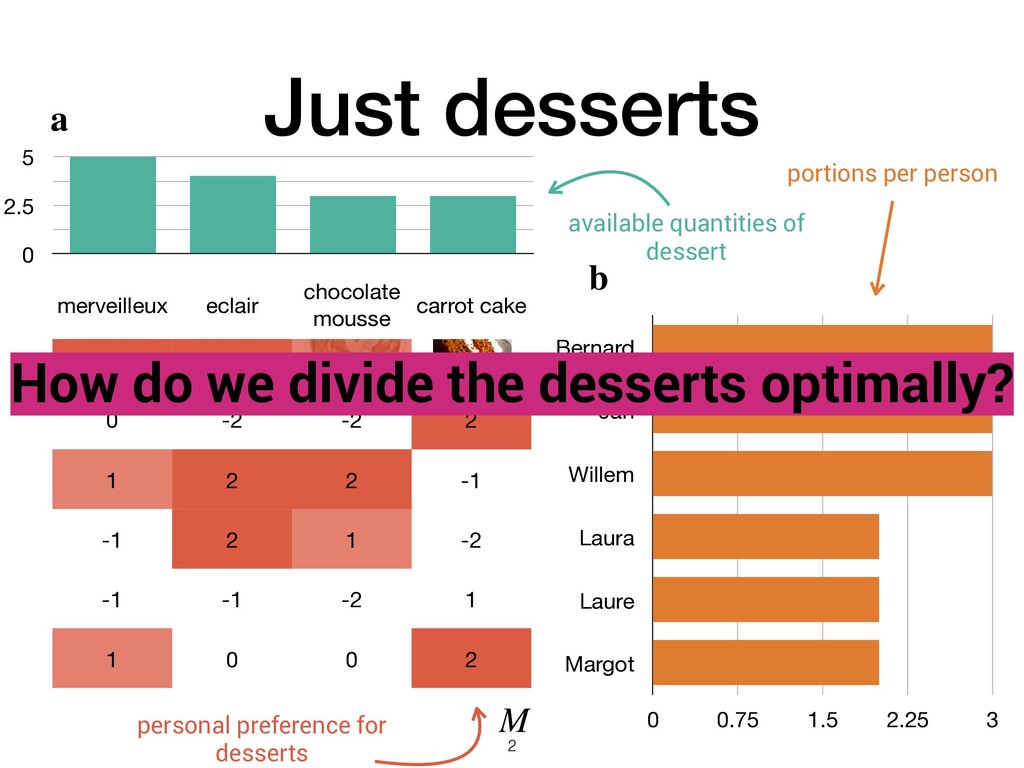
2. Just desserts 0 2.5 5 available quantities of dessert Bernard Jan Willem Laura Laure Margot 0 0.75 1.5 2.25 3 portions per person merveilleux eclair chocolate mousse carrot cake 2 2 1 0 0 -2 -2 2 1 2 2 -1 -1 2 1 -2 -1 -1 -2 1 1 0 0 2 personal preference for desserts How do we divide the desserts optimally? a b M 2
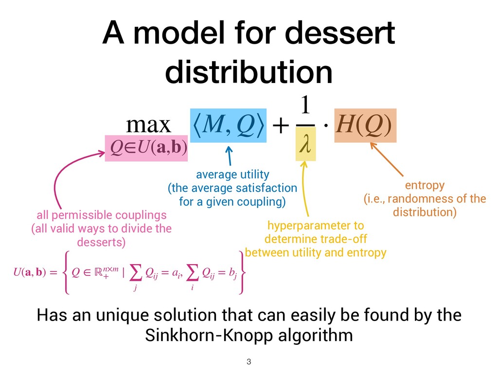
3. A model for dessert distribution max Q∈U(a,b) ⟨M, Q⟩ + 1 λ ⋅ H(Q) average utility (the average satisfaction for a given coupling) hyperparameter to determine trade-off between utility and entropy entropy (i.e., randomness of the distribution) 3 all permissible couplings (all valid ways to divide the desserts) U(a, b) = Q ∈ ℝn×m + ∣ ∑ j Qij = ai , ∑ i Qij = bj Has an unique solution that can easily be found by the Sinkhorn-Knopp algorithm
4. Couplings and effect of λ 4
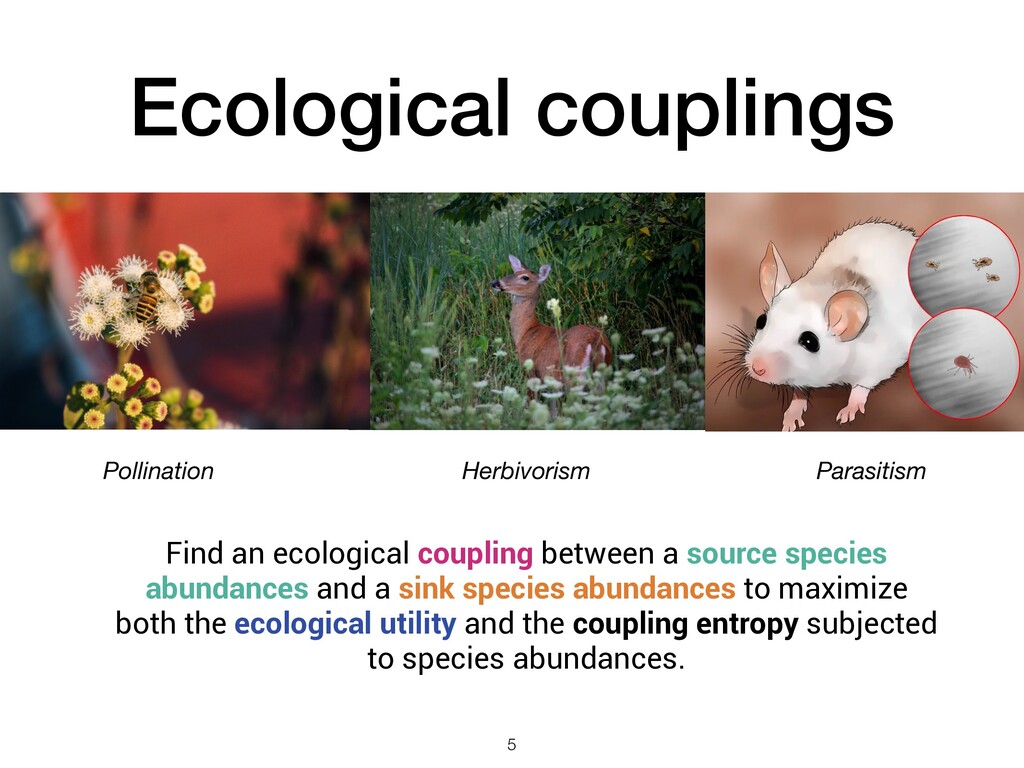
5. Ecological couplings Pollination Herbivorism Parasitism Find an ecological coupling between a source species abundances and a sink species abundances to maximize both the ecological utility and the coupling entropy subjected to species abundances. 5
6. Trait matching example 25 50 75 100 125 10 20 30 40 P plant sp. pol. sp. 0 0.005 0.010 0.015 0.020 0.025 0.030 0.035 0.040 25 50 75 100 125 10 20 30 40 Q plant sp. pol. sp. 0.005 0.010 0.015 0.020 0.025 0.030 25 50 75 100 125 10 20 30 40 M plant sp. pol. sp. 0 0.1 0.2 0.3 0.4 0.5 0.6 0.7 0.8 0.9 1.0 10- 3 10- 2 10- 1 100 1.25 1.25 1.26 1.26 1.27 1.27 Kullback- Leibler divergence (nats) optimal transport neutral Observed coupling Utility matrix using trait matching Predicted coupling using abundances 6
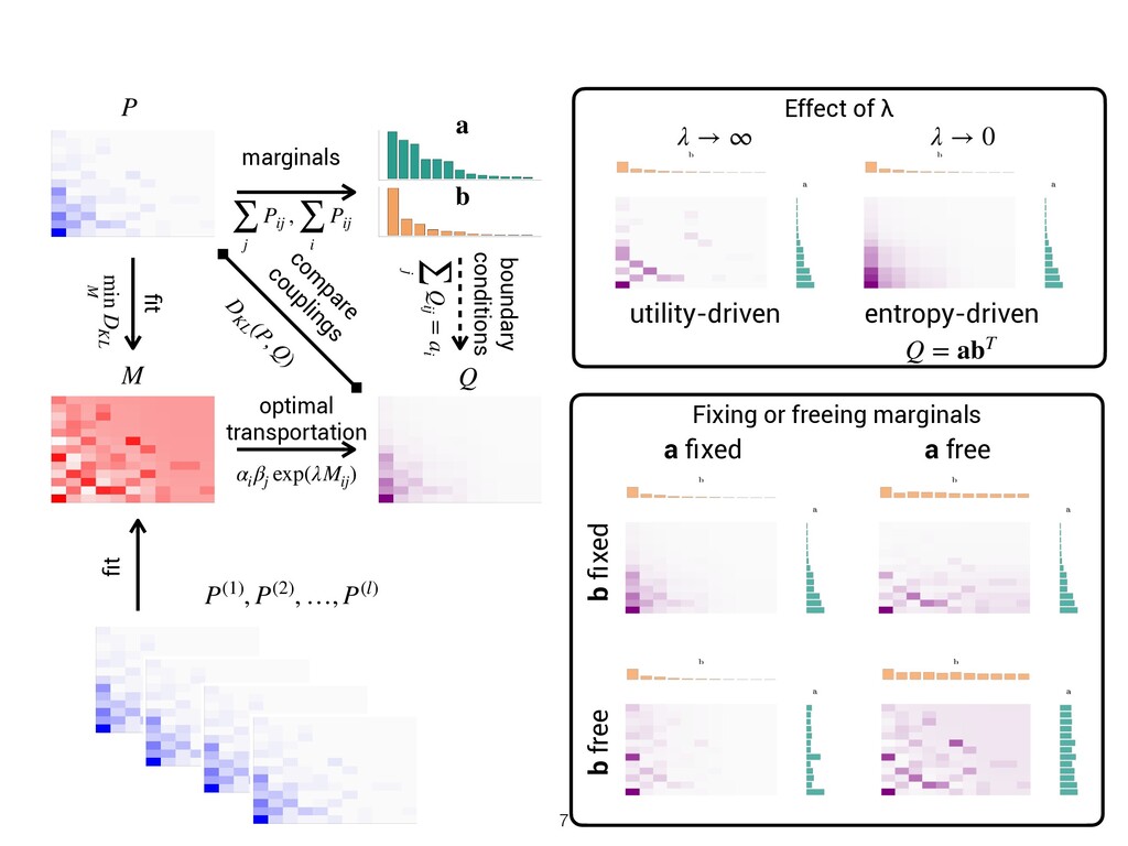
7. P Effect of λ utility-driven entropy-driven Q = abT λ → ∞ λ → 0 D KL (P,Q ) com pare couplings a b marginals ∑ j Pij , ∑ i Pij boundary conditions optimal transportation αi βj exp(λMij ) ∑ j Qij = ai Q M Fixing or freeing marginals a fixed a free b fixed b free fit min M DKL P(1), P(2), …, P(l) fit 7
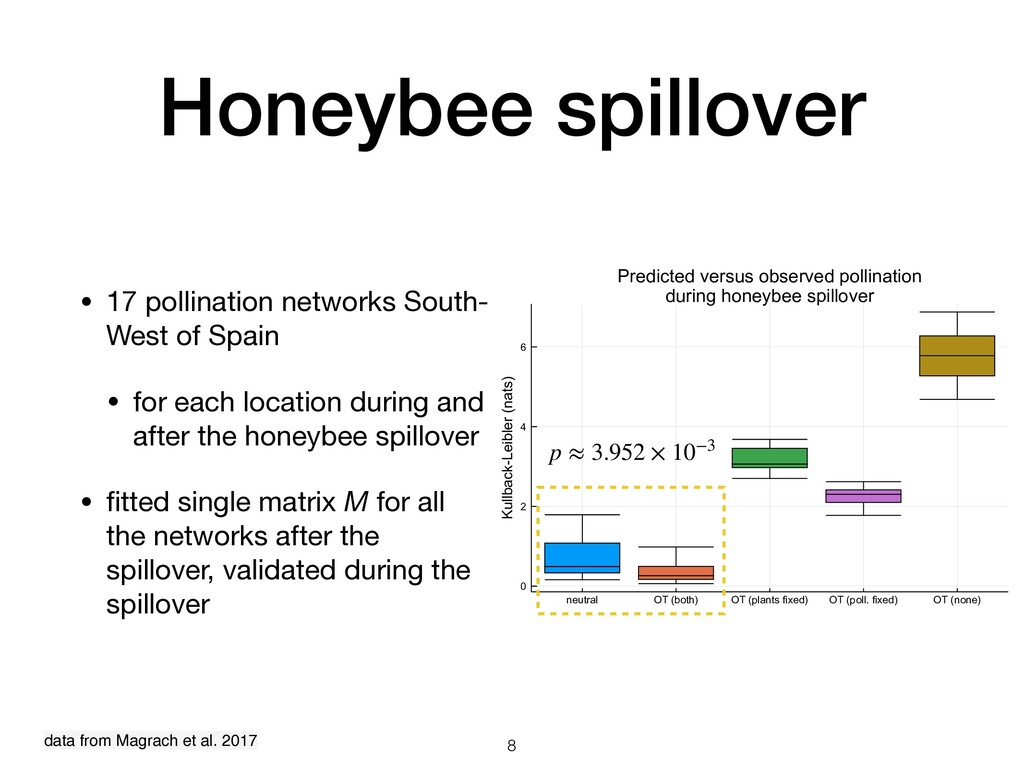
8. Honeybee spillover • 17 pollination networks South- West of Spain • for each location during and after the honeybee spillover • fitted single matrix M for all the networks after the spillover, validated during the spillover neutral OT (both) OT (plants fixed) OT (poll. fixed) OT (none) 0 2 4 6 Predicted versus observed pollination during honeybee spillover Kullback-Leibler (nats) data from Magrach et al. 2017 p ≈ 3.952 × 10−3 8
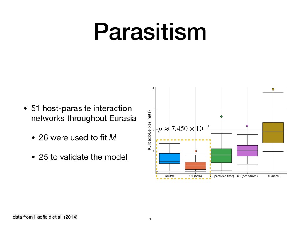
9. neutral OT (both) OT (parasites fixed) OT (hosts fixed) OT (none) 0 1 2 3 4 Kullback-Leibler (nats) Parasitism • 51 host-parasite interaction networks throughout Eurasia • 26 were used to fit M • 25 to validate the model data from Hadfield et al. (2014) p ≈ 7.450 × 10−7 9
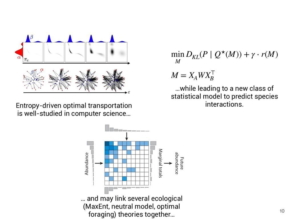
10. Entropy-driven optimal transportation is well-studied in computer science… … and may link several ecological (MaxEnt, neutral model, optimal foraging) theories together… M = XA WX⊤ B min M DKL (P ∣ Q⋆(M)) + γ ⋅ r(M) …while leading to a new class of statistical model to predict species interactions. 10