Upgrade to Pro — share decks privately, control downloads, hide ads and more …

Modelling the effect of lockdown

Modelling the effect of lockdown

The note consists of two parts.
In a crude analysis, we have seen that the growth rate in the number of daily confirmed cases is roughly linear in activity index(from the mobility report of apple).
In a refined analysis, we have seen that while SEIR model does not reproduce the data well, SEIR model with time delay reproduces the data well. Furthermore, it is suspected the ratio of $\beta$(growth rate of number of daily confirmed cases) before and after lockdown might be square of the ratio of activity index before and after lockdown. We need to further examine the relation of $\beta$ and activity index in order to predict the number of confirmed cases.

mistecon

May 06, 2020
Tweet

More Decks by mistecon

Other Decks in Science

Transcript

  1. Modelling the effect of lockdown 2020-5-6 1 Introduction Due to

    the worldwide pandemic of COVID-19, many countries are trying to slow down the spreading of the virus through lockdown of the cities. At the time of writing this (2020/4/29) some has already achieved dramatic decrease in the number of patients, while most of them are still struggling, therefore it is crucial to evaluate the effect of the lockdown, equivalently, to estimate the time the lockdown is needed. Therefore, we will try to model the dynamics for the number of patients, considering the effect of lockdown. We have roughly two different type of mod- els which could explain the dynamics, one is ordinary SEIR type of model as in [1], in which transfer from one state to another is proportional to the number of original state, and another is SEIR type of model which includes the effect of time delay[2]. In this model, once someone gets infected, they will become contagious and later quarantined after fixed period of time1. Using actual num- ber of patients[5] and the activity data from mobile phone[6], we wish to know which type of model better describes the reality. In the second section, we briefly describe the structure of two types of models, and in the third section we will see the overview of the model and fitting of the models with the real data. In the final section we will examine the result and possible future developments. 2 Model Let me describe two types of models of contagion. The ordinary SEIR type of model we consider here consists of 5(or 4 for simplicity) states. S: suscepti- ble(not infected), E: Exposed(infected but not yet contagious) I:Infected(infected and contagious) Q:Quarantined(infected but separated from others) R:Recovered(infected but recovered and no more contagious). Naturally the population of those 5 states adds up to the total number of population N. We assume that the trans- fer from state S to state E is proportional to S and I, because the infection 1In reality, we know that the time infected person becomes contagious is rather fixed[3], and also it will take a while since patients go to a doctor till they receive the result of PCR testing. Therefore we expect the model with time delay will describe the dynamics better. 1
  2. happens via the contact of people in these two states.

    We further assume the transfer from E to I is proportional to the number of E(therefore it is somewhat similar to the decay of a particle to another state), and transfer from I to Q and I to R are also proportional to the number of people in state I. Figure 1: Transfer between states in SEIR model and delayed model. Therefore, denoting the number of people in that particular state as the same letter, we would have a combination of equations ˙ S = −β(t) S(t)I(t) N ˙ E = β(t) S(t)I(t) N − γE(t) ˙ I = γE(t) − (δ1 + δ2 )I(t) ˙ Q = δ1 I(t) ˙ R = δ2 I(t). (1) The parameter in the model can be estimated by following clinical consid- eration; Since it is known one will be infectious after 3 to 5 days after the infection, the time scale for transferring from E to I can be estimated to be around 42. Time scale for transfer from I to Q can be estimated to be around 1 week considering the situation in Japan[4], but expected to vary from country to country. The transfer parameter δ2 from state I to state R is expected to be around 1/14, because it is considered it takes about two weeks for COVID-19 to be cured(to become not infectious). Another type of model is SEIR type of model with delay in time and the equations are given as below. 2The time from infection till one becomes symptomatic is around 5 days as in the study in Diamond Princess[3]and it is also known that one can be infectious 1 ∼ 2 days before one becomes symptomatic[7]. Therefore time scale for this process is 4 and γ should be around 0.25, 2
  3. ˙ S = −β(t) S(t) N I(t) ˙ E =

    β(t) S(t) N I(t) − β(t − τ) S(t − τ) N I(t − τ) ˙ I = β(t − τ) S(t − τ) N I(t − τ) − aβ(t − τ2 ) S(t − τ2 ) N I(t − τ2 ) − (1 − a)β(t − τ3 ) S(t − τ3 ) N I(t − τ3 ) ˙ Q = aβ(t − τ2 ) S(t − τ2 ) N I(t − τ2 ) ˙ R = (1 − a)β(t − τ3 ) S(t − τ3 ) N I(t − τ3 ). (2) In reality, once you get infected with coronavirus, becoming symptomatic and being tested positive happens after certain amount of time rather than happening at certain probability. If transfer from S to E happens at time t, transfer from state E to state I happens at time t + τ, where τ ∼ 4, and assuming that state I will proceed to state Q with probability a and to state R with probability (1 − a), we further assume that the transfer from state I to state Q will happen at time t − τ2 and I to R at time t − τ3 . 3 Data After brief description on the datasets, we will perform two different data anal- ysis to know which of the two models above describe the dynamics of confirmed cases better including the effect of lockdown. We use the data for the confirmed cases from ourworlddata.org[5] and mobility data from apple mobility report[6]. The apple mobility report records how many times people searched for certain path using apple map, and the number of search is counted for car, walk and transit respectively. In the first analysis, we wish to know the time lag from infection to quar- antine (τ2 ) heuristically. If the value of β and S is constant, the growth rate3 of I should be proportional to β. Therefore, naively, we could expect that the growth rate of Q should be the same, so we might expect that the value of β and growth rate of ˙ Q(= daily confirmed cases) is proportional. We have changed the value of τ2 and performed the linear regression of growth rate of ˙ Q(t) with respect to β(t − τ2 ), and computed p-value for each regression. There are roughly 5 countries which has already achieved the drastic decrease in the number of confirmed cases and data is available, Australia, Austria, Czech, Norway and Switzerland. We would focus on those 5 countries. Among those, please take a look at figures for Australia and Austria below. First figure shows the number of confirmed cases, and the second shows the growth rate of 3We computed the slope of confirmed cases with respect to time as the growth rate. 3
  4. the number of confirmed cases and activity index taken by

    [6]4. In the third figure, growth rate in confirmed cases and activity 12 days before was plotted. Figure 2: daily confirmed cases in Australia Figure 3: activity index and growth rate of confirmed cases in Australia Figure 4: activity index(12 days before) and growth rate of confirmed cases in Aus- tralia Figure 5: daily confirmed cases in Austria Figure 6: activity index and growth rate of confirmed cases in Austria Figure 7: activity index(12 days before) and growth rate of confirmed cases in Austria You can see that the growth rate changes according to the change of activity index with around 10 days of delay. We have also performed linear regression on growth rate of confirmed cases and activity index, changing the time lag τ. As a result, we will have p-value for the regression and we have plotted the log(p-value) in the figure (8). If we interpret the location of minimum p-value as the most probable model5, we can conclude τ ∼ 12. In the next step, let’s perform two types of simulation I have described, SEIR type model and SEIR type model with delay. In this part, we simplify the analysis for ease of analysis. Here we ignore the state R because it is a bit hard to know the ratio of patients who will not quarantined but be cured without any treatment. For the former model, we have variables the number of people for S,E,I,Q, and total number of people N, and transfer coefficients γ, δ are given by medical consideration. We will fit the model to the data by tuning I0 (I at certain time), and the value of β. We naively expect the value of β to be proportional to activity index, but then it will not match the observation. We then assume that 4In the original database, the distance people searched through apple map for walk, drive, transit are recorded and we just took the average of these indices as activity index. 5If possible we should compare the model of different τ by free energy or BIC, but we don’t have time to do that. 4
  5. Figure 8: log(p-value) of linear regression of growth rate of

    confirmed cases with respect to activity index, changing time lag τ the time dependence of β is similar to that of activity index. That is, as in Fig.9, we first approximate the dynamics of activity index as constant for t < t1 and t > t2 , and linearly decrease for t1 < t ≦ t2 . We then assume that β is constant for t < t1 and t > t2 , and linearly decrease for t1 < t ≦ t2 . Figure 9: Time dependence of activity and the value of β. In the delayed SEIR model, we instead have N and τ from clinical consid- eration, because it is known that the time period from infection till one gets infectious is considered to be around 4 days. We then fit the model to daily confirmed cases and obtain τ2 , β0 , β1 , I0 . If we wish to see log( ˙ Q), I0 corresponds to the intercept of the line, β0 corresponds to the slope of the line, τ2 corresponds to the time of lockdown, and β1 corresponds to the slope of the line after lockdown, so it is not so hard to estimate the value of the parameters. Here we adjust those parameters by hand and saw the value of ˙ Q for actual and model. Here we show plot of those together 5
  6. with the plot of β. For Australia, the parameter for

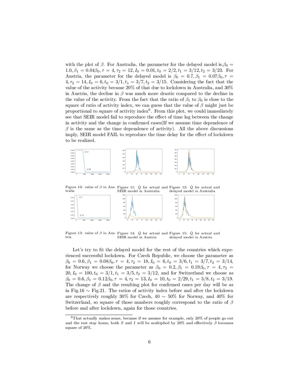
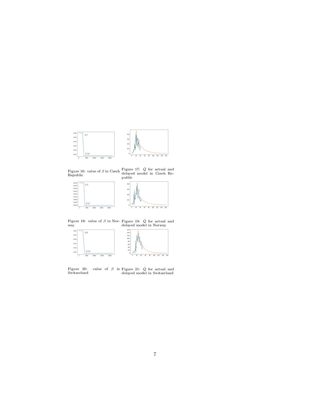
    the delayed model is,β0 = 1.0, β1 = 0.04β0 , τ = 4, τ2 = 12, I0 = 0.01, t0 = 2/2, t1 = 3/12, t2 = 3/23. For Austria, the parameter for the delayed model is β0 = 0.7, β1 = 0.07β0 , τ = 4, τ2 = 14, I0 = 6, t0 = 3/1, t1 = 3/7, t2 = 3/15. Considering the fact that the value of the activity became 20% of that due to lockdown in Australia, and 30% in Austria, the decline in β was much more drastic compared to the decline in the value of the activity. From the fact that the ratio of β1 to β0 is close to the square of ratio of activity index, we can guess that the value of β might just be proportional to square of activity index6. From this plot, we could immediately see that SEIR model fail to reproduce the effect of time lag between the change in activity and the change in confirmed cases(If we assume time dependence of β is the same as the time dependence of activity). All the above discussions imply, SEIR model FAIL to reproduce the time delay for the effect of lockdown to be realized. Figure 10: value of β in Aus- tralia Figure 11: ˙ Q for actual and SEIR model in Australia Figure 12: ˙ Q for actual and delayed model in Australia Figure 13: value of β in Aus- tria Figure 14: ˙ Q for actual and SEIR model in Austria Figure 15: ˙ Q for actual and delayed model in Austria Let’s try to fit the delayed model for the rest of the countries which expe- rienced successful lockdown. For Czech Republic, we choose the parameter as β0 = 0.6, β1 = 0.08β0 , τ = 4, τ2 = 18, I0 = 6, t0 = 3/6, t1 = 3/7, t2 = 3/14, for Norway we choose the parameter as β0 = 0.2, β1 = 0.19β0 , τ = 4, τ2 = 20, I0 = 100, t0 = 3/1, t1 = 3/5, t2 = 3/12, and for Switzerland we choose as β0 = 0.6, β1 = 0.12β0 , τ = 4, τ2 = 13, I0 = 10, t0 = 2/29, t1 = 3/8, t2 = 3/19. The change of β and the resulting plot for confirmed cases per day will be as in Fig.16 ∼ Fig.21. The ratios of activity index before and after the lockdown are respectively roughly 30% for Czech, 40 ∼ 50% for Norway, and 40% for Switzerland, so square of those numbers roughly correspond to the ratio of β before and after lockdown, again for those countries. 6That actually makes sense, because if we assume for example, only 20% of people go out and the rest stay home, both S and I will be multiplied by 20% and effectively β becomes square of 20%. 6
  7. Figure 16: value of β in Czech Republic Figure 17:

    ˙ Q for actual and delayed model in Czech Re- public Figure 18: value of β in Nor- way Figure 19: ˙ Q for actual and delayed model in Norway Figure 20: value of β in Switzerland Figure 21: ˙ Q for actual and delayed model in Switzerland 7
  8. 4 Conclusion and Discussion In the above discussion, as a

    crude data analysis, we have seen that growth rate of confirmed cases of COVID-19 is roughly linear in activity index, with time delay around 10 ± 5 days. In a more refined data analysis, we have tried to fit to the data with SEIR model and similar model with time delay and seen that it is not likely SEIR fits the real data, while the model with time delay can reproduce the data. Furthermore, it is interesting that the ratio of β before and after lockdown, β1 /β0 , is close to the value of square of ratio of activity index before and after lockdown. It would be meaningful to see the general relation between the ratio of β and ratio of activity index. Knowing that, we would be able to predict the number of confirmed cases after lockdown. References [1] Hethcote, Herbert W. ”The mathematics of infectious diseases.” SIAM re- view 42, no. 4 (2000): 599-653. [2] COVID-19 ৘ใڞ༗ ʕ COVID19-Information sharing, ౎ಓ෎ݝ͝ͱͷγ ϛϡϨʔγϣϯʹΑΔݕ౼, Sato, Aki-Hiro, et al. ”An epidemic simulation with a delayed stochastic SIR model based on international socioeconomic- technological databases.” 2015 IEEE International Conference on Big Data (Big Data). IEEE, 2015. [3] Mizumoto, Kenji, et al. ”Estimating the asymptomatic proportion of coro- navirus disease 2019 (COVID-19) cases on board the Diamond Princess cruise ship, Yokohama, Japan, 2020.” Eurosurveillance 25.10 (2020). [4] ”Suspected patients wait up to a week to get tested ”, https://www3.nhk.or.jp/nhkworld/en/news/20200417_33/ [5] https://ourworldindata.org/coronavirus [6] https://www.apple.com/covid19/mobility [7] Wei, Wycliffe E. ”Presymptomatic Transmission of SARS-CoV-2ʕ Singapore, January 23–March 16, 2020.” MMWR. Morbidity and Mortality Weekly Report 69 (2020). 8