Anthropomorphic image reconstruction via optimal control and hypoelliptic diffusion

by U. Boscain

Transcript

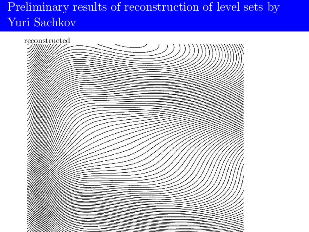
1. Anthropomorphic Image Reconstruction via Optimal Control and Hypoelliptic Diffusion Ugo Boscain CNRS, CMAP, Ecole Polytechnique, Paris, France and INRIA team GECO Jean-Paul Gauthier, LSIS, Toulon Dario Prandi, Paris Dophine Alexei Remizov, CMAP, Ecole Polytechnique Roman Chertovskih, Universidade do Porto work supported by the ERC grant GECOMETHODS December 3, 2015
2. An algorithm of image reconstruction based on a model of the mammals visual cortex V1 65% of corruption
3. 85% of corruption
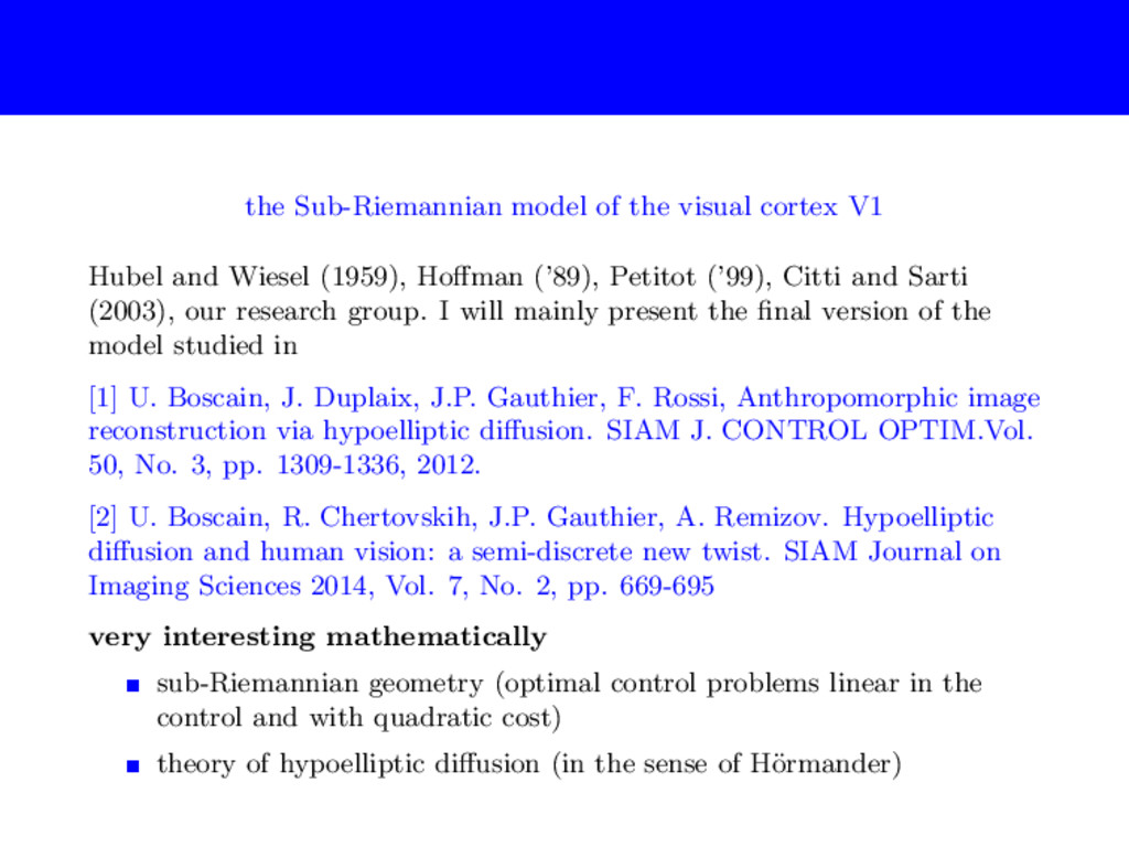
4. the Sub-Riemannian model of the visual cortex V1 Hubel and Wiesel (1959), Hoffman (’89), Petitot (’99), Citti and Sarti (2003), our research group. I will mainly present the final version of the model studied in [1] U. Boscain, J. Duplaix, J.P. Gauthier, F. Rossi, Anthropomorphic image reconstruction via hypoelliptic diffusion. SIAM J. CONTROL OPTIM.Vol. 50, No. 3, pp. 1309-1336, 2012. [2] U. Boscain, R. Chertovskih, J.P. Gauthier, A. Remizov. Hypoelliptic diffusion and human vision: a semi-discrete new twist. SIAM Journal on Imaging Sciences 2014, Vol. 7, No. 2, pp. 669-695 very interesting mathematically sub-Riemannian geometry (optimal control problems linear in the control and with quadratic cost) theory of hypoelliptic diffusion (in the sense of H¨ ormander)
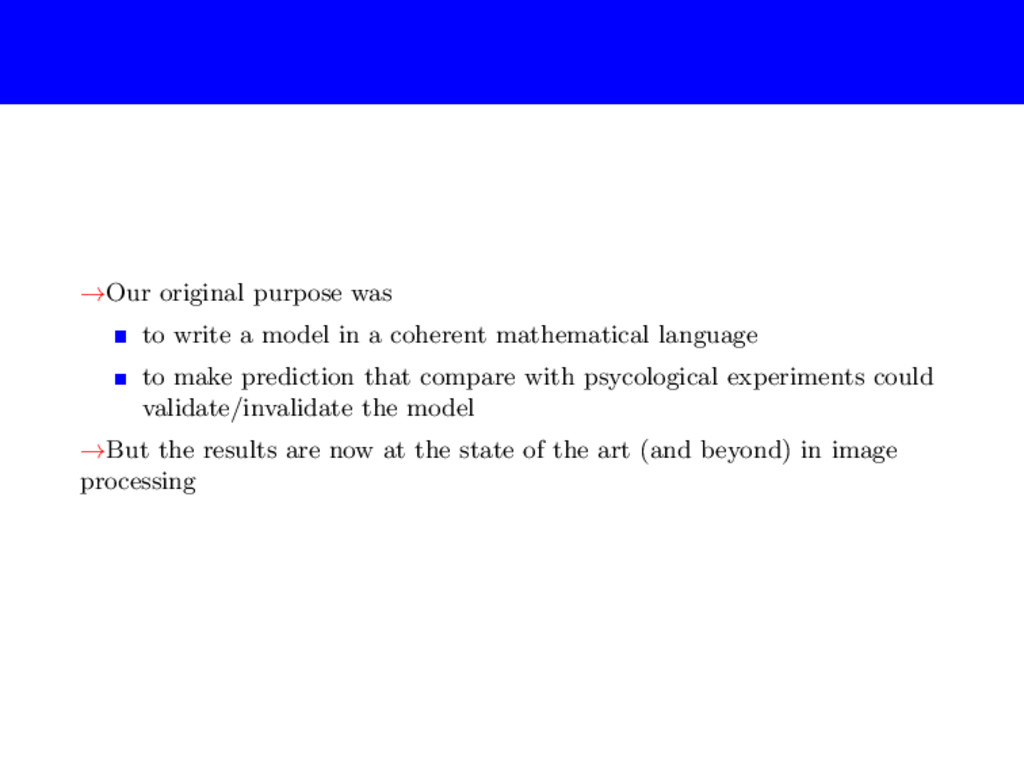
5. →Our original purpose was to write a model in a coherent mathematical language to make prediction that compare with psycological experiments could validate/invalidate the model →But the results are now at the state of the art (and beyond) in image processing
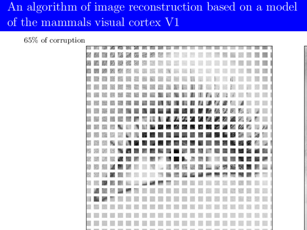
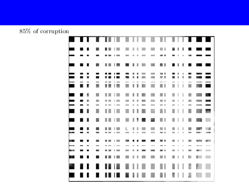
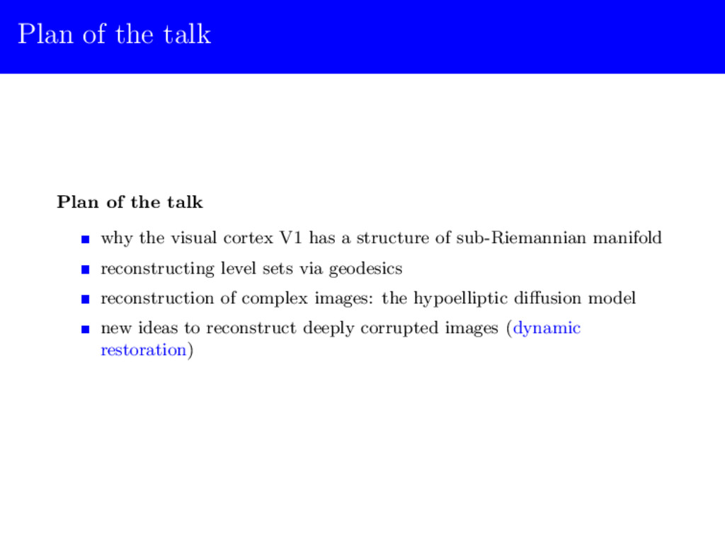
6. Plan of the talk Plan of the talk why the visual cortex V1 has a structure of sub-Riemannian manifold reconstructing level sets via geodesics reconstruction of complex images: the hypoelliptic diffusion model new ideas to reconstruct deeply corrupted images (dynamic restoration)
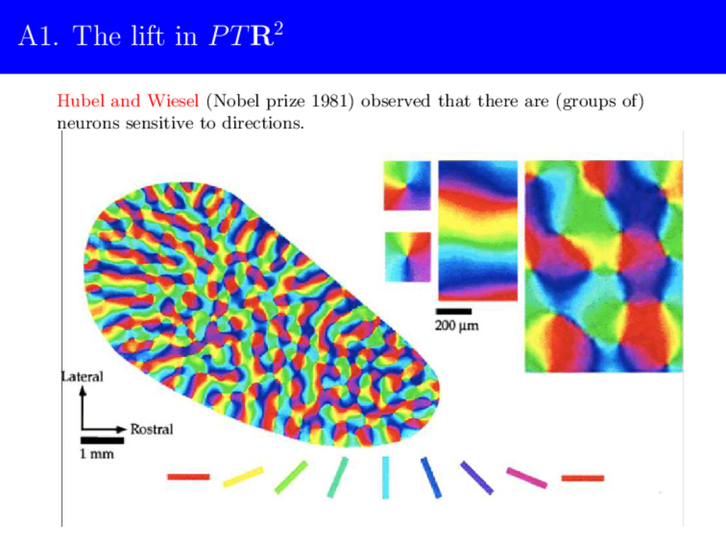
7. Two ideas coming from neurophyology of the visual cortex V1 A. Hubel and Wiesel (1959) observed that there are (groups of) neurons sensitive to positions and directions. Hence the visual cortex lifts an image on the PT R2 = R2 × P1 (experimental fact) B. an image is reconstructed by minimizing the energy necessary to excite groups of neurons that are not excited by the image in PT R2 (postulate)
8. A1. The lift in PTR2 Hubel and Wiesel (Nobel prize 1981) observed that there are (groups of) neurons sensitive to directions.
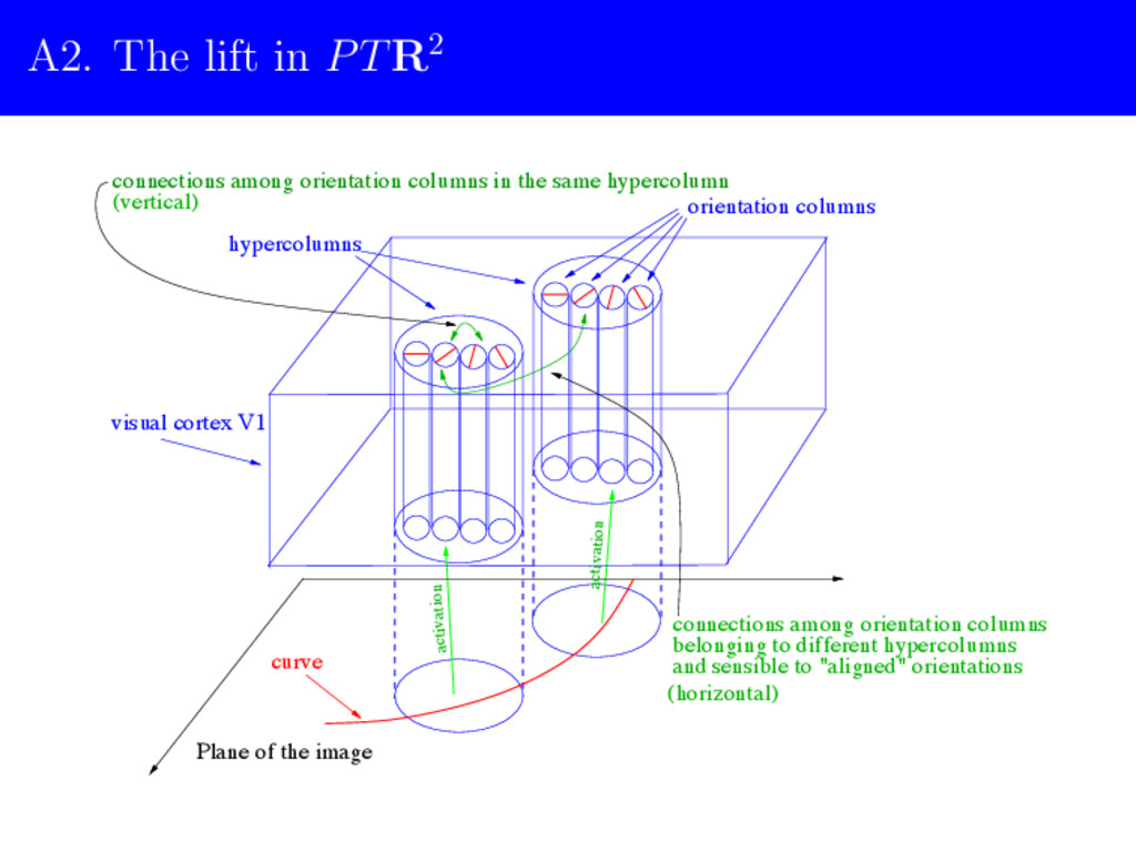
9. A2. The lift in PTR2 and sensible to "aligned" orientations curve visual cortex V1 activation activation orientation columns Plane of the image connections among orientation columns in the same hypercolumn (vertical) hypercolumns connections among orientation columns belonging to different hypercolumns (horizontal)
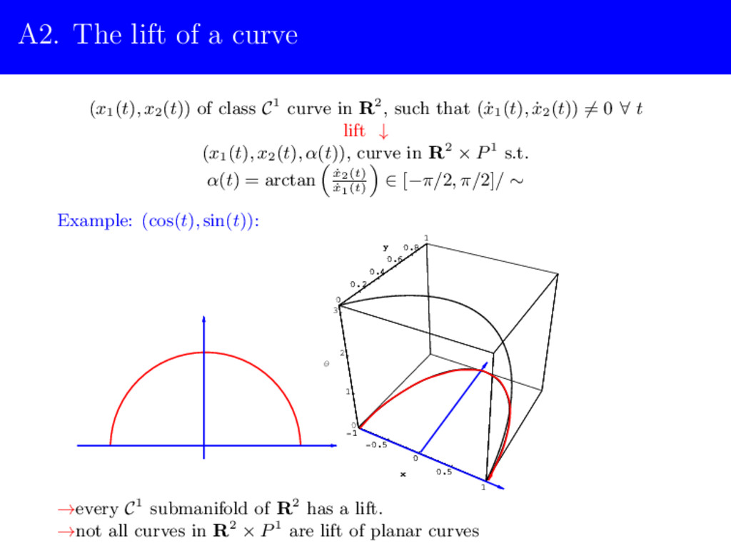
10. A3. The lift in PTR2 the visual cortex stores an image as a set of points and tangent directions, i.e. it makes a lift to PT R2 = R2 × P1. The projective tangent bundle of R2 (or bundle of directions of the plane). π/2 x2 α ∈ [0, π]/ ∼ α x1 P1 −π/2 PT R2 can be seen as a fiber bundle whose base is R2 and whose fiber at the point (x1, x2) is the set of straight lines (i.e. directions without orientation) d(x1,x2) attached to (x1, x2).
11. A2. The lift of a curve (x1(t), x2(t)) of class C1 curve in R2, such that ( ˙ x1(t), ˙ x2(t)) ̸= 0 ∀ t lift ↓ (x1(t), x2(t), α(t)), curve in R2 × P1 s.t. α(t) = arctan ˙ x2(t) ˙ x1(t) ∈ [−π/2, π/2]/ ∼ Example: (cos(t), sin(t)): -1 -0.5 0 0.5 1 x 0 0.2 0.4 0.6 0.8 1 y 0 1 2 3 Θ -1 -0.5 0 0.5 x 0 0.2 0.4 0.6 0.8 y →every C1 submanifold of R2 has a lift. →not all curves in R2 × P1 are lift of planar curves
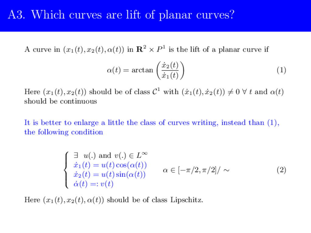
12. A3. Which curves are lift of planar curves? A curve in (x1(t), x2(t), α(t)) in R2 × P1 is the lift of a planar curve if α(t) = arctan ˙ x2(t) ˙ x1(t) (1) Here (x1(t), x2(t)) should be of class C1 with ( ˙ x1(t), ˙ x2(t)) ̸= 0 ∀ t and α(t) should be continuous It is better to enlarge a little the class of curves writing, instead than (1), the following condition ⎧ ⎪ ⎪ ⎨ ⎪ ⎪ ⎩ ∃ u(.) and v(.) ∈ L∞ ˙ x1(t) = u(t) cos(α(t)) ˙ x2(t) = u(t) sin(α(t)) ˙ α(t) =: v(t) α ∈ [−π/2, π/2]/ ∼ (2) Here (x1(t), x2(t), α(t)) should be of class Lipschitz.
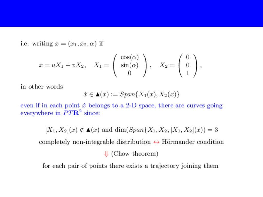
13. i.e. writing x = (x1, x2, α) if ˙ x = uX1 + vX2, X1 = ⎛ ⎝ cos(α) sin(α) 0 ⎞ ⎠ , X2 = ⎛ ⎝ 0 0 1 ⎞ ⎠ , in other words ˙ x ∈ (x) := Span{X1(x), X2(x)} even if in each point ˙ x belongs to a 2-D space, there are curves going everywhere in PT R2 since: [X1, X2](x) / ∈ (x) and dim(Span{X1, X2, [X1, X2](x)) = 3 completely non-integrable distribution ↔ H¨ ormander condition ⇓ (Chow theorem) for each pair of points there exists a trajectory joining them
14. B1. How V1 reconstruct an interrupted curve 2 γ ( ) γ ( ) b c 0 0 x x 1 Consider a smooth curve γ0 : [a, b] ∪ [c, d] → R2, interrupted in ]b, c[. We want to complete γ0 by a curve γ : [b, c] → R2 that is: γ(b) = γ0(b), γ(c) = γ0(c) ˙ γ(b) ∼ ˙ γ0(b) ̸= 0, ˙ γ(c) ∼ ˙ γ0(c) ̸= 0. we assume γ(b) ̸= γ(c), ˙ γ0(b) ̸= 0, ˙ γ0(c) ̸= 0
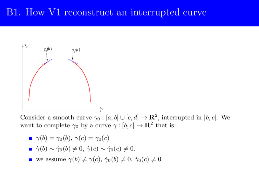
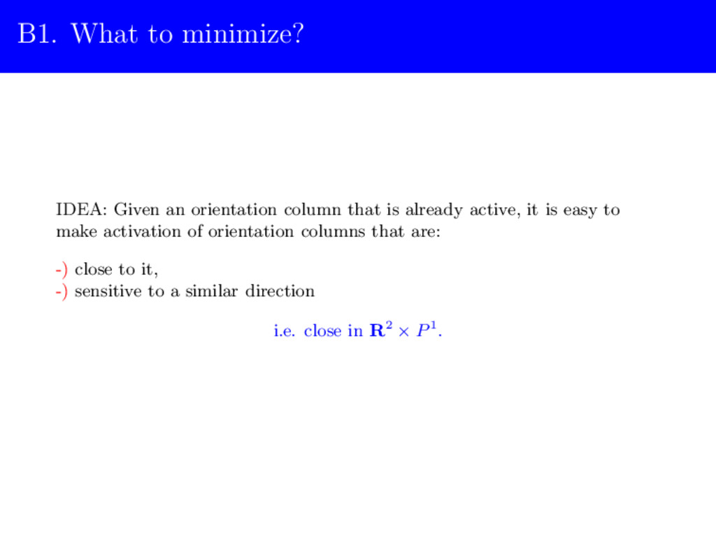
15. B1. What to minimize? IDEA: Given an orientation column that is already active, it is easy to make activation of orientation columns that are: -) close to it, -) sensitive to a similar direction i.e. close in R2 × P1.
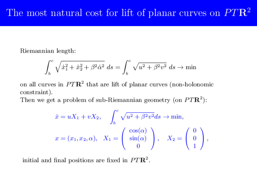
16. The most natural cost for lift of planar curves on PTR2 Riemannian length: c b ˙ x2 1 + ˙ x2 2 + β2 ˙ α2 ds = c b u2 + β2v2 ds → min on all curves in PT R2 that are lift of planar curves (non-holonomic constraint). Then we get a problem of sub-Riemannian geometry (on PT R2): ˙ x = uX1 + vX2, c b u2 + β2v2ds → min, x = (x1, x2, α), X1 = ⎛ ⎝ cos(α) sin(α) 0 ⎞ ⎠ , X2 = ⎛ ⎝ 0 0 1 ⎞ ⎠ , initial and final positions are fixed in PT R2.
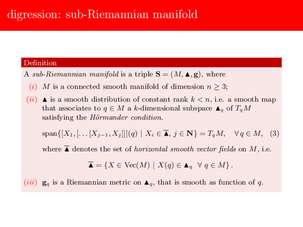
17. digression: sub-Riemannian manifold Definition A sub-Riemannian manifold is a triple S = (M, , g), where (i) M is a connected smooth manifold of dimension n ≥ 3; (ii) is a smooth distribution of constant rank k < n, i.e. a smooth map that associates to q ∈ M a k-dimensional subspace q of Tq M satisfying the H¨ ormander condition. span{[X1, [. . . [Xj−1, Xj ]]](q) | Xi ∈ , j ∈ N} = Tq M, ∀ q ∈ M, (3) where denotes the set of horizontal smooth vector fields on M, i.e. = {X ∈ Vec(M) | X(q) ∈ q ∀ q ∈ M} . (iii) gq is a Riemannian metric on q , that is smooth as function of q.
18. A Lipschitz continuous curve γ : [0, T ] → M is said to be horizontal if ˙ γ(t) ∈ γ(t) for a.e. t ∈ [0, T ]. Given an horizontal curve γ : [0, T ] → M, the length of γ is l(γ) = T 0 g(˙ γ, ˙ γ) dt. (4)
19. horizontal curve (q) The distance induced by the sub-Riemannian structure on M is the function d(q0, q1) = inf{l(γ) | γ(0) = q0, γ(T ) = q1, γ horizontal}. (5) The hypothesis of connectedness of M and the H¨ ormander ⇒ →the finiteness and the continuity of d(·, ·) with respect to the topology of M (Chow’s Theorem) →The function d(·, ·) is called the Carnot-Caratheodory distance and gives to M the structure of metric space.
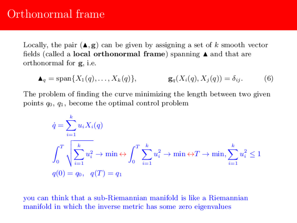
20. Orthonormal frame Locally, the pair ( , g) can be given by assigning a set of k smooth vector fields (called a local orthonormal frame) spanning and that are orthonormal for g, i.e. q = span{X1(q), . . . , Xk (q)}, gq (Xi (q), Xj (q)) = δij . (6) The problem of finding the curve minimizing the length between two given points q0, q1, become the optimal control problem ˙ q = k i=1 ui Xi (q) T 0 k i=1 u2 i → min ↔ T 0 k i=1 u2 i → min ↔T → min, k i=1 u2 i ≤ 1 q(0) = q0, q(T ) = q1 you can think that a sub-Riemannian manifold is like a Riemannian manifold in which the inverse metric has some zero eigenvalues
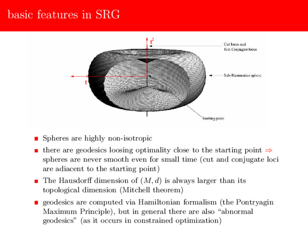
21. basic features in SRG t2 t Spheres are highly non-isotropic there are geodesics loosing optimality close to the starting point ⇒ spheres are never smooth even for small time (cut and conjugate loci are adiacent to the starting point) The Hausdorff dimension of (M, d) is always larger than its topological dimension (Mitchell theorem) geodesics are computed via Hamiltonian formalism (the Pontryagin Maximum Principle), but in general there are also “abnormal geodesics” (as it occurs in constrained optimization)
22. Lot of open questions for instance regularity of minimizers: in (n − 1, n) they are smooth, but in larger co-dimension it is not known topology of small balls: it is not know if they are homeomorphic to euclidean balls see the book “A tour of sub-Riemannian geometry” by R. Montgomery the lecture notes “Introduction to Riemannian and sub-Riemannian geometry” Agrachev, Barilari, B.
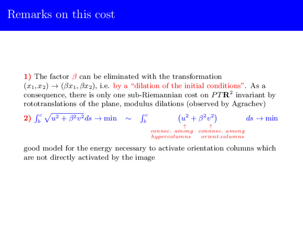
23. Remarks on this cost 1) The factor β can be eliminated with the transformation (x1, x2) → (βx1, βx2), i.e. by a “dilation of the initial conditions”. As a consequence, there is only one sub-Riemannian cost on PT R2 invariant by rototranslations of the plane, modulus dilations (observed by Agrachev) 2) c b u2 + β2v2ds → min ∼ c b u2 + β2v2 ↑ ↑ connec. among connnec. among hypercolumns orient.columns ds → min good model for the energy necessary to activate orientation columns which are not directly activated by the image
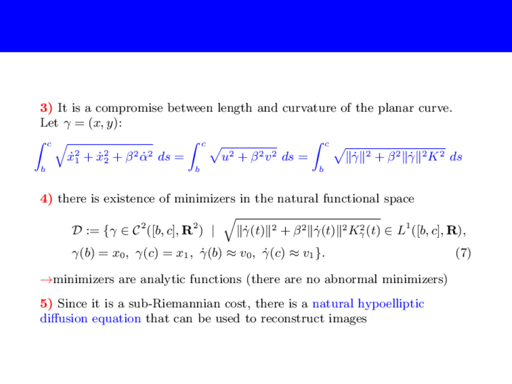
24. 3) It is a compromise between length and curvature of the planar curve. Let γ = (x, y): c b ˙ x2 1 + ˙ x2 2 + β2 ˙ α2 ds = c b u2 + β2v2 ds = c b ∥˙ γ∥2 + β2∥˙ γ∥2K2 ds 4) there is existence of minimizers in the natural functional space D := {γ ∈ C2([b, c], R2) | ∥˙ γ(t)∥2 + β2∥˙ γ(t)∥2K2 γ (t) ∈ L1([b, c], R), γ(b) = x0, γ(c) = x1, ˙ γ(b) ≈ v0, ˙ γ(c) ≈ v1}. (7) →minimizers are analytic functions (there are no abnormal minimizers) 5) Since it is a sub-Riemannian cost, there is a natural hypoelliptic diffusion equation that can be used to reconstruct images
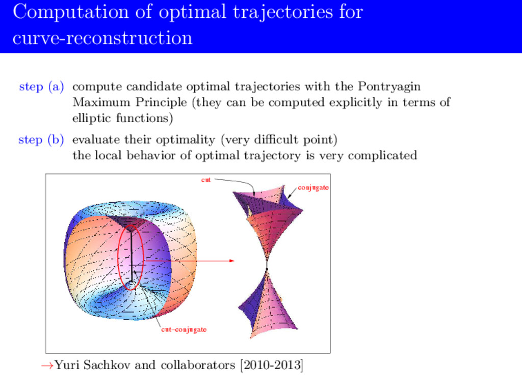
25. Computation of optimal trajectories for curve-reconstruction step (a) compute candidate optimal trajectories with the Pontryagin Maximum Principle (they can be computed explicitly in terms of elliptic functions) step (b) evaluate their optimality (very difficult point) the local behavior of optimal trajectory is very complicated cut cut−conjugate conjugate →Yuri Sachkov and collaborators [2010-2013]
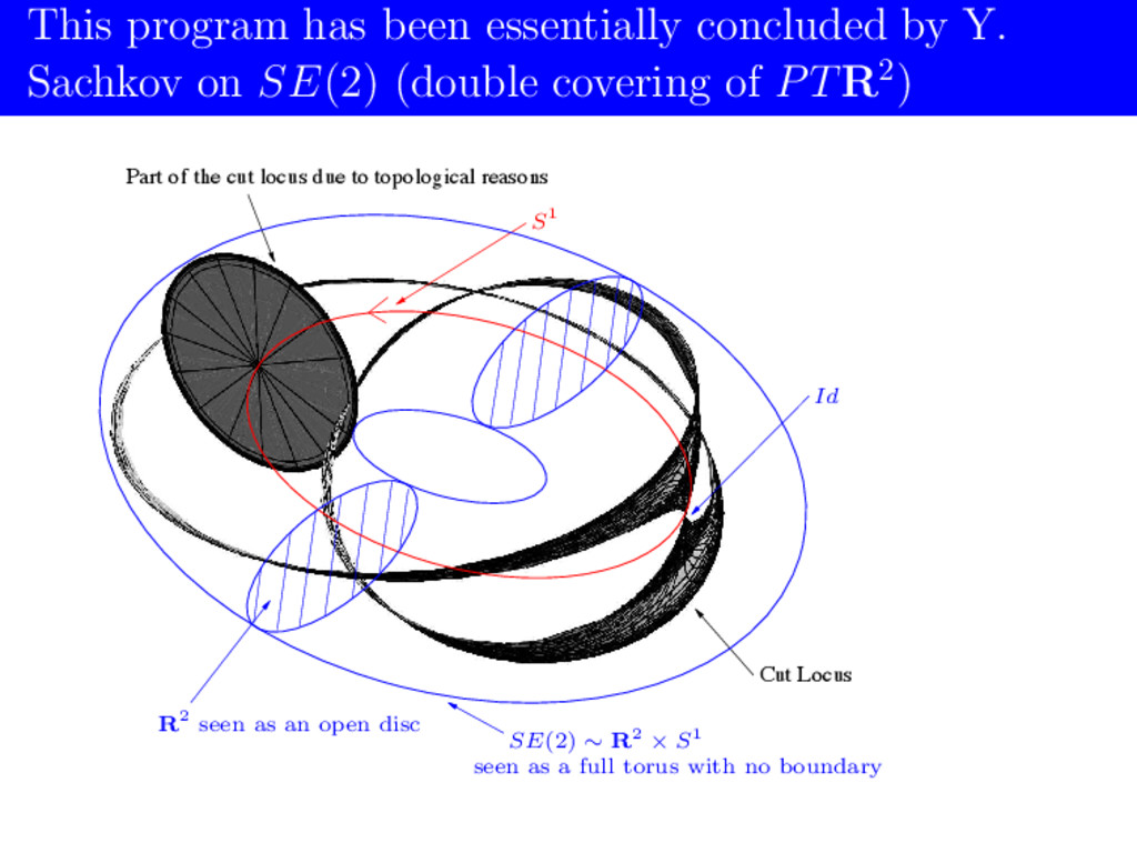
26. This program has been essentially concluded by Y. Sachkov on SE(2) (double covering of PTR2) Cut Locus Part of the cut locus due to topological reasons seen as a full torus with no boundary Id R2 seen as an open disc S1 SE(2) ∼ R2 × S1
27. Preliminary results of reconstruction of level sets by Yuri Sachkov and his group Original
28. Preliminary results of reconstruction of level sets by Yuri Sachkov corrupted
29. Preliminary results of reconstruction of level sets by Yuri Sachkov reconstructed
30. Complex images (not just a simple contour): ? ? ?
31. An idea to reconstruct images all possible paths are activated as a Brownian motion For instance: dx = X1dW1 + X2dW2, → ∂t ψ(t, x) = (X1 2 + X2 2)ψ(t, x) X1 2 + X2 2 = (cos(α)∂x1 + sin(α)∂x2 )2 + β2∂2 α (sub-elliptic Heat equation, under H¨ ormander condition ⇒ solutions are smooth) The diffusion is highly non isotropic ∂t ψ(t, x) = (X1 2 + X2 2)ψ(t, x) −t log Pt (x, y) → − d(x, y)2 4t Varadhan-Leandre
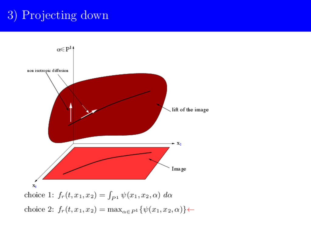
32. PLAN: Let I : R2 → [0, 1] be the image 0) smoothing the image with a Gaussian (it is made by the eyes) to get well defined level sets fc = I ∗ G(σx , σy ) ∈ L2(R2, R) ∩ C∞(R2, R), generically we get a Morse function. See: [1] Boscain, J. Duplaix, J.P. Gauthier, F. Rossi, SIAM SICON 2012 1) lifting the image to PT R2 and using it as an initial condition for the hypoelliptic heat eq. In the same paper we proved that the lift of a Morse function is a smooth surface in PT R2 2) computing the hypoelliptic diffusion ← 3) projecting down the image
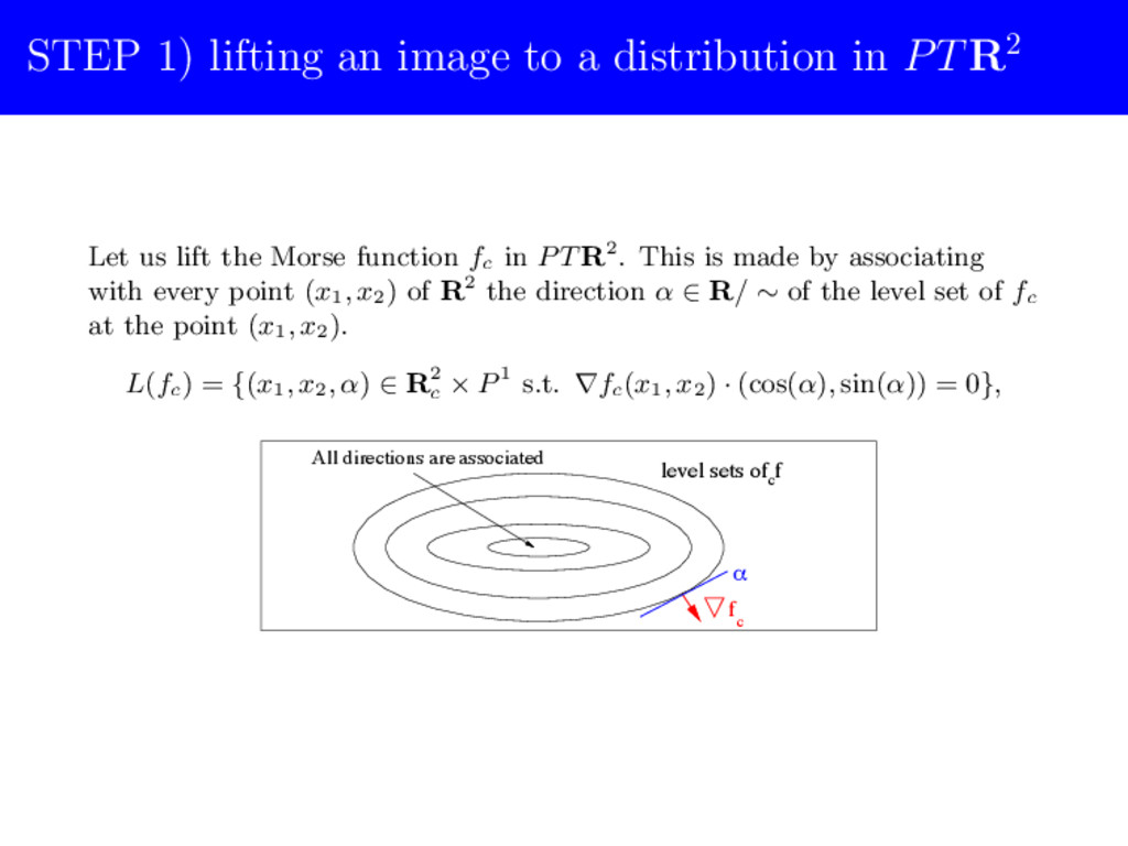
33. STEP 1) lifting an image to a distribution in PTR2 Let us lift the Morse function fc in PT R2. This is made by associating with every point (x1, x2) of R2 the direction α ∈ R/ ∼ of the level set of fc at the point (x1, x2). L(fc ) = {(x1, x2, α) ∈ R2 c × P1 s.t. ∇fc (x1, x2) · (cos(α), sin(α)) = 0}, c level sets of f All directions are associated α c f
34. Define the distribution on R × P1: ˆ fc (x1, x2, α) = fc (x1, x2)δ(d((x1, x2, α), L(f)) α 1 P smoothing Image lift of the image x x1 (distribution supported in L(f)) 2 corrupted part Ω
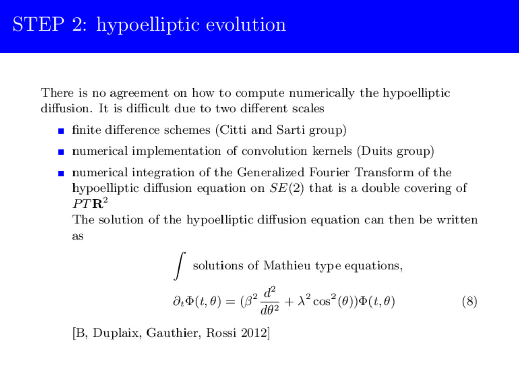
35. STEP 2: hypoelliptic evolution There is no agreement on how to compute numerically the hypoelliptic diffusion. It is difficult due to two different scales finite difference schemes (Citti and Sarti group) numerical implementation of convolution kernels (Duits group) numerical integration of the Generalized Fourier Transform of the hypoelliptic diffusion equation on SE(2) that is a double covering of PT R2 The solution of the hypoelliptic diffusion equation can then be written as solutions of Mathieu type equations, ∂t Φ(t, θ) = (β2 d2 dθ2 + λ2 cos2(θ))Φ(t, θ) (8) [B, Duplaix, Gauthier, Rossi 2012]
36. 3) Projecting down non isotropic diffusion 1 2 x x Image lift of the image α 1 P choice 1: fr (t, x1, x2) = P 1 ψ(x1, x2, α) dα choice 2: fr (t, x1, x2) = maxα∈P 1 {ψ(x1, x2, α)}←
37. →This algorithm does not use the knowledge of where the image is corrupted (it is not an inpainting problem)
38. Dynamic restoration Can we do more by using the information of where the image is corrupted to work on images as ? (85% of corrupted pixels)
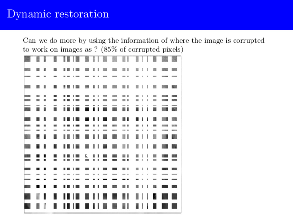
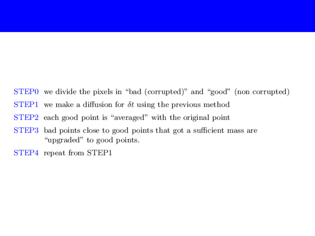
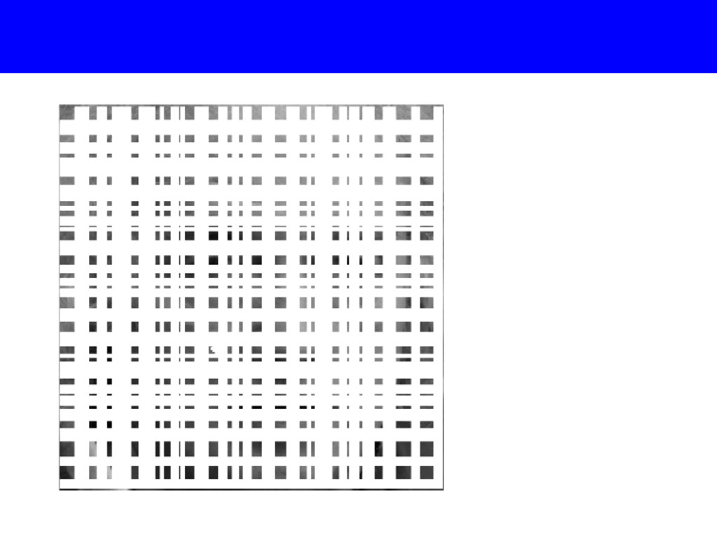
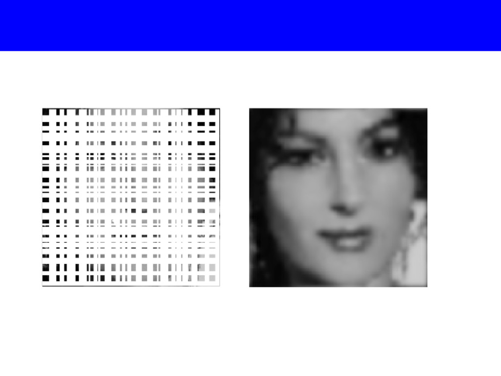
39. STEP0 we divide the pixels in “bad (corrupted)” and “good” (non corrupted) STEP1 we make a diffusion for δt using the previous method STEP2 each good point is “averaged” with the original point STEP3 bad points close to good points that got a sufficient mass are “upgraded” to good points. STEP4 repeat from STEP1
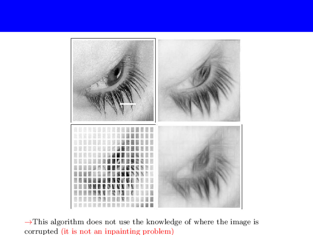
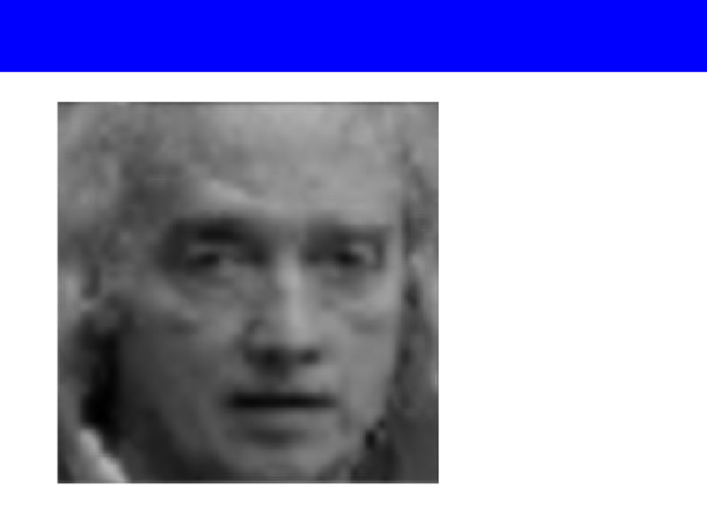
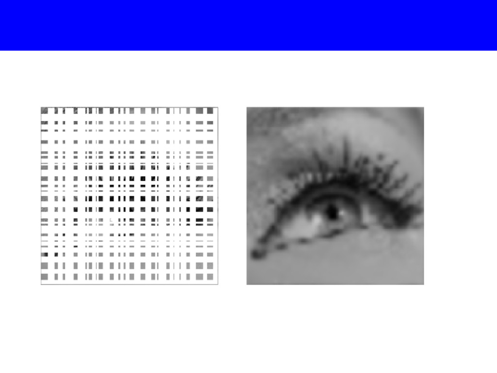
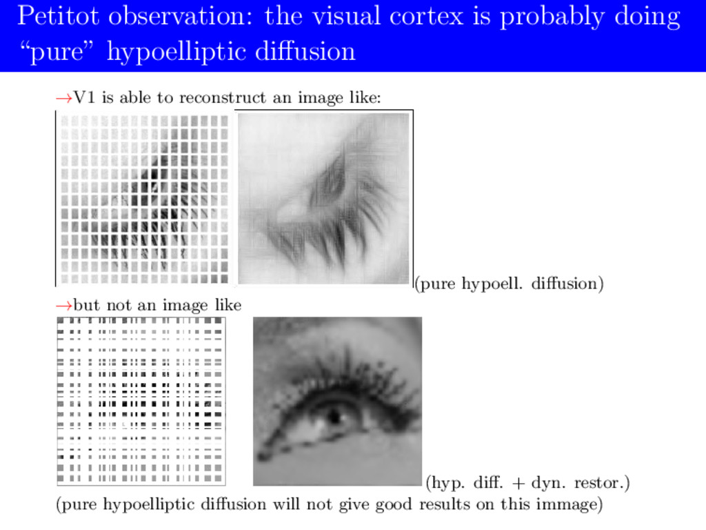
44. Petitot observation: the visual cortex is probably doing “pure” hypoelliptic diffusion →V1 is able to reconstruct an image like: (pure hypoell. diffusion) →but not an image like (hyp. diff. + dyn. restor.) (pure hypoelliptic diffusion will not give good results on this immage)
45. The END