Earth-Moon Lyapunov to Lyapunov Mission: Long Time Duration, Low-Thrust Transfer

by M. Chupin

Transcript

1. Earth-Moon Lyapunov to Lyapunov Mission: Low Thrust Transfer Maxime Chupin Thomas Haberkorn, Emmanuel Trélat GdR MOA 2015 (Dijon) 3rd of December 2015
2. M. Chupin — Interplanetary Transfer with Low Consumption Outline 1/26 • Three Body Problem – Lyapunov Orbits – Invariant Manifolds • The Mission – Optimal Control Problem – Using Invariant Manifolds
3. M. Chupin — Interplanetary Transfer with Low Consumption Circular Restricted 3 Body Problem 2/26 Rotating coordinate system in which the two primaries are fixed (along the axis). In this work Earth-Moon system. A satellite with negligible mass . 2 primaries 1 and 2 rotating around their center of mass. Respective mass: 1 and 2. d d = −1 13 3 13 − 2 23 3 23 Normalize the system: distance ′ = ∗ , velocity ′ = ∗ , time ′ = u∗ 2u . The mass parameter: = 2 1 + 2 . 1 2
4. M. Chupin — Interplanetary Transfer with Low Consumption Normalized System 3/26 State: = (, , ̇ , ̇ )u = (1 , 2 , 3 , 4 )u , ⎧ { { { { { { ⎨ { { { { { { ⎩ ̇ 1 = 3 ̇ 2 = 4 ̇ 3 = 1 + 24 − (1 − ) 1 − 0 1 3 1 − 1 − 0 2 3 2 ̇ 4 = 2 − 23 − (1 − ) 2 3 1 − 2 3 2 ⇔ ⎧ { { { { { ⎨ { { { { { ⎩ ̇ 1 = 3 = 1 () ̇ 2 = 4 = 2 () ̇ 3 = 24 − 1 = 3 () ̇ 4 = −23 − 2 = 4 () where 1 = √(1 − 0 1 )2 + 2 2 and 2 = √(1 − 0 2 )2 + 2 2 are respectively the distances between and primaries 1 and 2. Potential: (1 , 2 ) = − 1 2 (2 1 + 2 2 ) − 1 − 1 − 2 − 1 2 (1 − ) . ̇ = 0 ().
5. M. Chupin — Interplanetary Transfer with Low Consumption Lagrange Points 4/26 2 3 1 4 5 2 1 Five equilibrium points called Lagrange points. Collinear points: 1, 2 and 3. Equilateral points: 4 and 5. Stability is studied by linearization. 1, 2 and 3 are instable. Stability of 4 and 5 depends on the system.
6. M. Chupin — Interplanetary Transfer with Low Consumption Lyapunov Orbits 5/26 The Lyapunov-Poincaré theorem ensures that a family of periodic orbits exists around Lagrange points. Method based on symmetry. Newton method. Initialization with analytical approximation (Richardson 80). −0.1−5 ⋅ 10−2 0 5 ⋅ 10−2 0.1 −0.4 −0.2 0 0.2 0.4 1 There exist 0 and u s.t. ⎧ { { ⎨ { { ⎩ (0 ) = 0 , (0 ) = 0, ̇ (0 ) = 0, ̇ (0 ) = ̇ 0 , and ⎧ { { ⎨ { { ⎩ (0 + u /2) = 1 , (0 + u /2) = 0, ̇ (0 + u /2) = 0, ̇ (0 + u /2) = ̇ 1 . Taking 0 = 0, we define the shooting function: ⟹ u (u , ̇ 0 ) = ( 2 (u /2, 0 ) 3 (u /2, 0 ) ) = ( 0 0 ) .
7. M. Chupin — Interplanetary Transfer with Low Consumption Family of Lyapunov Orbits 6/26 Continuation method: define a family of problems u, such that 0 is easy to solve, and 1 is the problem we want to solve. Initialization of uu with solution of uu−1 . We have solved the problem for a given ℰ0. We want to reach a certain energy ℰ1. −0.1−5 ⋅ 10−2 0 5 ⋅ 10−2 0.1 −0.4 −0.2 0 0.2 0.4 1 Continuation problems: ℰ u ∶ u ℰ (u , 0 , ̇ 0 ) = ⎛ ⎜ ⎜ ⎜ ⎝ 2 (u /2, 0 ) 3 (u /2, 0 ) ℰ(0 ) − ℰu ⎞ ⎟ ⎟ ⎟ ⎠ = ⎛ ⎜ ⎜ ⎜ ⎝ 0 0 0 ⎞ ⎟ ⎟ ⎟ ⎠ where ℰ(0 ) is the energy of the trajectory starting at 0 = (0 , 0, 0, ̇ 0 ) and ℰu = (1 − )ℰ0 + ℰ1 .
8. M. Chupin — Interplanetary Transfer with Low Consumption Invariant Manifolds 7/26 Definition: A stable manifold (resp. instable) of a periodic orbit is the set of the phase space consisting of all points whose future (resp. past) semi-orbits converge to it (asymptotic orbits). (Koon et al., 2006) 0 u+ u+ u−(0 ) u+(0 ) u−(0 ) u+(0 ) ̄ (⋅) periodic solution with period s.t. ̄ (0) = ̄ 0. The monodromy matrix for the point ̄ 0: = (; ̄ 0 ) 0 Local approximation with particular eigenvectors.
9. M. Chupin — Interplanetary Transfer with Low Consumption Invariant Manifolds 8/26 Definition: A stable manifold (resp. instable) of a periodic orbit is the set of the phase space consisting of all points whose future (resp. past) semi-orbits converge to it (asymptotic orbits). (Koon et al., 2006) 0.6 0.4 0.2 0 0.2 0.4 0.6 0.5 0 0.5 L1 x y ̄ (⋅) periodic solution with period s.t. ̄ (0) = ̄ 0. The monodromy matrix for the point ̄ 0: = (; ̄ 0 ) 0 . Local approximation with particular eigenvectors. Sort of gravitationnal currents.
10. M. Chupin — Interplanetary Transfer with Low Consumption Invariant Manifolds 9/26
11. M. Chupin — Interplanetary Transfer with Low Consumption The Mission 10/26 From one Lyapunov orbit around 1 to another Lyapunov orbit around 2 with low thrust: 0.8 0.9 1 1.1 1.2 −0.1 0 0.1 Moon 1 2 The controlled dynamics: ⎧ { { ⎨ { { ⎩ ̇ = 0 () + 2 ∑ u=1 u u (), ̇ = −∗ || , 1 = ⎛ ⎜ ⎜ ⎜ ⎜ ⎜ ⎜ ⎝ 0 0 1 0 ⎞ ⎟ ⎟ ⎟ ⎟ ⎟ ⎟ ⎠ and 2 = ⎛ ⎜ ⎜ ⎜ ⎜ ⎜ ⎜ ⎝ 0 0 0 1 ⎞ ⎟ ⎟ ⎟ ⎟ ⎟ ⎟ ⎠ , where ∈ ℝ2, || ⩽ 1, is the maximal thrust, ∗ is a constant modeling the engines. Controllability: see (Caillau, Daoud 2012). Similar mission: (Epenoy 2012).
12. M. Chupin — Interplanetary Transfer with Low Consumption Optimal Control Problem 11/26 Tools: Use Pontryagin’s Maximum Principle (PMP). Shooting Method. Continuation Method. 0.8 0.9 1 1.1 1.2 −0.1 0 0.1 ∗ 0 ∗ 3 Moon 1 2 u ⎧ { { { { { { { ⎨ { { { { { { { ⎩ u = min ∫ uu 0 ‖‖2 d, ̇ = 0 () + 2 ∑ u=1 u u (), ̇ = −∗ || , || ≤ 1, (0) ∈ Lya1 , and (u ) ∈ Lya2 , (0) = 0 .
13. M. Chupin — Interplanetary Transfer with Low Consumption Heteroclinic Orbit 12/26 0.8 0.9 1 1.1 1.2 −0.1 0 0.1 2 3 Moon 1 2 0.8 0.9 1 1.1 1.2 −0.1 0 0.1 Moon 1 2 0.8 0.85 0.9 0.95 1 1.05 1.1 1.15 1.2 −0.1 −5 · 10−2 0 5 · 10−2 0.1 U2 U3 Moon L1 L2 x −0.1 −6 ⋅ 10−2 −2 ⋅ 10−2 −2 0 2 4 6 ̇
14. M. Chupin — Interplanetary Transfer with Low Consumption Transfer Lya 1 to Het 13/26 u1 ⎧ { { { { { { { ⎨ { { { { { { { ⎩ min ∫ u0 0 ‖‖2 d, ̇ = 0 () + 2 ∑ u=1 u u (), ̇ = −∗ || , || ≤ 1, (0) = ∗ 0 , (0) = ∗ 0 , (0 ) = ∗ 1 . Application PMP: Hamiltonian: ℋ(, , , u , ), normal case. Maximization condition gives : (, , , u ). ((0), u (0)) ? Lya1 = argmin u∈Lya1 ∥u1 Het − ∥. Propagate backwards Lya1 during Lya1 : ⟶ ∗ 0 . Propagate forward Het during u1 Het : ⟶ ∗ 1 . 0 = Lya1 + u1 Het . Shooting function: u1 ((0), u (0)) = ⎛ ⎜ ⎝ ext 1,…,4 (0 , ∗ 0 , ∗ 0 , (0), u (0)) − ∗ 1 ext 10 (0 , ∗ 0 , ∗ 0 , (0), u (0)) ⎞ ⎟ ⎠
15. M. Chupin — Interplanetary Transfer with Low Consumption Transfer Lya 1 to Het 14/26 u u1 ⎧ { { { { { { { { ⎨ { { { { { { { { ⎩ min ∫ u0 0 ‖‖2 d, ̇ = 0 () + 2 ∑ u=1 u u (), ̇ = −∗ || , || ≤ 1, (0) = ∗ 0 , (0) = ∗ 0 , (0 ) = u 1 = (1 − )nat Lya1 + ∗ 1 . Continuation: ((0), u (0)) = 0 corresponds to the uncontrolled trajectory. Use solution of uu−1 u1 to initialize uu u1 . Lya1 u1 Het u1 Het • ∗ 0 ∈ Lya1 • ∗ 1 ∈ Het • nat Lya1 cont. Shooting function: u u1 ((0), u (0)) = ⎛ ⎜ ⎝ ext 1,…,4 (0 , ∗ 0 , ∗ 0 , (0), u (0)) − u 1 ext 10 (0 , ∗ 0 , ∗ 0 , (0), u (0)) ⎞ ⎟ ⎠
16. M. Chupin — Interplanetary Transfer with Low Consumption Transfer Lya 1 to Het 15/26 u u1 ⎧ { { { { { { { { ⎨ { { { { { { { { ⎩ min ∫ u0 0 ‖‖2 d, ̇ = 0 () + 2 ∑ u=1 u u (), ̇ = −∗ || , || ≤ 1, (0) = ∗ 0 , (0) = ∗ 0 , (0 ) = u 1 = (1 − )nat Lya1 + ∗ 1 . 0 1 2 3 −4 −2 0 2 ⋅10−6 1 () 0 1 2 3 −5 0 5 ⋅10−6 2 () 0 1 2 3 2 4 6 ⋅10−6 |()| Transfer Iterations Cost ↔ max Comp. Time 1 21 6.309 67 × 10−11 60 N 2.821 s Lya1 u1 Het u1 Het • ∗ 0 ∈ Lya1 • ∗ 1 ∈ Het • nat Lya1 cont.
17. M. Chupin — Interplanetary Transfer with Low Consumption Transfer Het to Lya 2 16/26 u u2 ⎧ { { { { { { { ⎨ { { { { { { { ⎩ min ∫ u2 0 ‖‖2 d, ̇ = 0 () + 2 ∑ u=1 u u (), ̇ = −∗ || , || ≤ 1, (0) = ∗ 2 , (0) = ∗ 2 , (0 ) = u 3 = (1 − )nat Het + ∗ 3 . 0 1 2 3 −1 0 1 ⋅10−5 1 () 0 1 2 3 0 2 ⋅10−5 2 () 0 1 2 3 1 2 3 ⋅10−5 |()| Transfer Iterations Cost ↔ max Comp. Time 2 19 9.061 24 × 10−10 60 N 1.439 s u2 Het Lya2 Lya2 • ∗ 2 ∈ Het • ∗ 3 ∈ Lya2 • nat Het cont.
18. M. Chupin — Interplanetary Transfer with Low Consumption Trajectory with Three Parts 17/26 0.8 0.85 0.9 0.95 1 1.05 1.1 1.15 1.2 −0.1 −8 ⋅ 10−2 −6 ⋅ 10−2 −4 ⋅ 10−2 −2 ⋅ 10−2 0 2 ⋅ 10−2 4 ⋅ 10−2 6 ⋅ 10−2 8 ⋅ 10−2 0.1 ∗ 0 ∗ 1 ∗ 2 ∗ 3 Moon 1 2
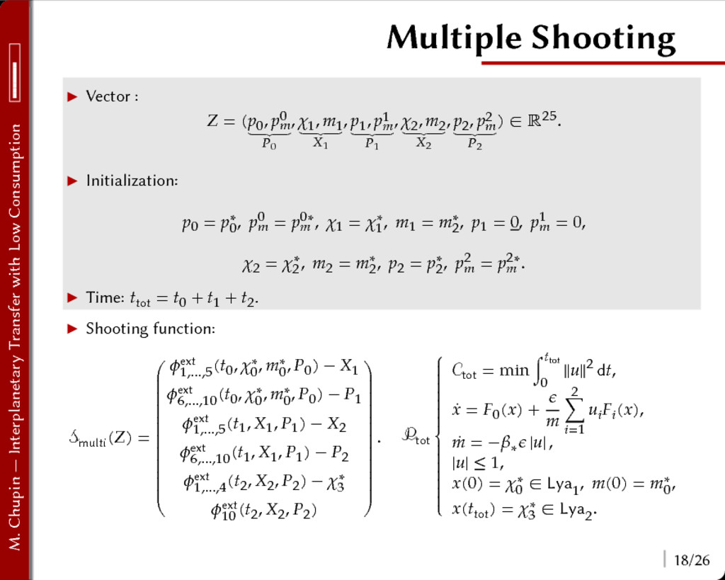
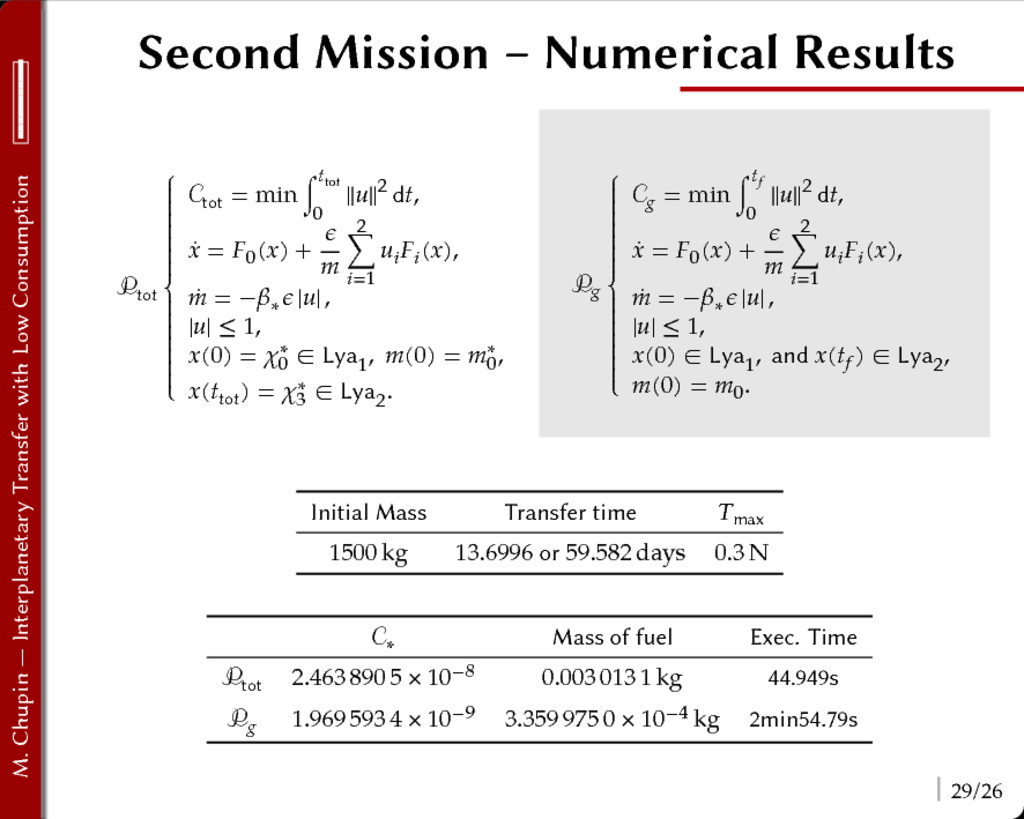
19. M. Chupin — Interplanetary Transfer with Low Consumption Multiple Shooting 18/26 Shooting function: multi () = ⎛ ⎜ ⎜ ⎜ ⎜ ⎜ ⎜ ⎜ ⎜ ⎜ ⎜ ⎜ ⎜ ⎜ ⎜ ⎜ ⎜ ⎜ ⎜ ⎜ ⎝ ext 1,…,5 (0 , ∗ 0 , ∗ 0 , 0 ) − 1 ext 6,…,10 (0 , ∗ 0 , ∗ 0 , 0 ) − 1 ext 1,…,5 (1 , 1 , 1 ) − 2 ext 6,…,10 (1 , 1 , 1 ) − 2 ext 1,…,4 (2 , 2 , 2 ) − ∗ 3 ext 10 (2 , 2 , 2 ) ⎞ ⎟ ⎟ ⎟ ⎟ ⎟ ⎟ ⎟ ⎟ ⎟ ⎟ ⎟ ⎟ ⎟ ⎟ ⎟ ⎟ ⎟ ⎟ ⎟ ⎠ . tot ⎧ { { { { { { { ⎨ { { { { { { { ⎩ tot = min ∫ utot 0 ‖‖2 d, ̇ = 0 () + 2 ∑ u=1 u u (), ̇ = −∗ || , || ≤ 1, (0) = ∗ 0 ∈ Lya1 , (0) = ∗ 0 , (tot ) = ∗ 3 ∈ Lya2 . Vector : = (0 , 0 u ⏟ u0 , 1 , 1 ⏟ u1 , 1 , 1 u ⏟ u1 , 2 , 2 ⏟ u2 , 2 , 2 u ⏟ u2 ) ∈ ℝ25. Initialization: 0 = ∗ 0 , 0 u = 0∗ u , 1 = ∗ 1 , 1 = ∗ 2 , 1 = 0, 1 u = 0, 2 = ∗ 2 , 2 = ∗ 2 , 2 = ∗ 2 , 2 u = 2∗ u . Time: tot = 0 + 1 + 2.
20. M. Chupin — Interplanetary Transfer with Low Consumption Thrust Continuation 19/26 60 N to help the multiple shooting continuation. Real thrust specification: e.g. 0.3 N. → continuation method. u = (1 − )0 + 1. u thrust ⎧ { { { { { { ⎨ { { { { { { ⎩ min ∫ utot 0 ‖‖2 d, ̇ = 0 () + u 2 ∑ u=1 u u (), ̇ = −∗ u || , || ≤ 1, (0) = ∗ 0 ∈ Lya1 , (0) = ∗ 0 , (tot ) = ∗ 3 ∈ Lya2 . With max = 60 N, the command does not reach 0.3 N. Continuation easy. Done with very few steps (22 in this case).
21. M. Chupin — Interplanetary Transfer with Low Consumption Trajectory 20/26 0.8 0.85 0.9 0.95 1 1.05 1.1 1.15 1.2 −0.1 −5 ⋅ 10−2 0 5 ⋅ 10−2 0.1 ∗ 0 ∗ 3 Moon 1 2
22. M. Chupin — Interplanetary Transfer with Low Consumption Optimal Command 21/26 0 5 10 −5 0 5 ⋅10−4 1 () (N) 0 5 10 −1 0 1 ⋅10−3 2 () (N) 0 5 10 0.5 1 ⋅10−3 |()| (N)
23. M. Chupin — Interplanetary Transfer with Low Consumption Optimization of Terminal Points 22/26 Pontryagin Maximum Principle applied to the general departure and arrival conditions (0) ∈ Lya1 and (u ) ∈ Lya2 gives us two transversality conditions: ⟨(0), 0 ((0))⟩ = 0 and ⟨(u ), 0 ((u ))⟩ = 0. 0 5 10 −2 −1 0 1 2 ⋅10−5 1 () (N) 0 5 10 0 0.5 1 ⋅10−5 2 () (N) 0 5 10 0 1 2 ⋅10−5 |()| (N)
24. M. Chupin — Interplanetary Transfer with Low Consumption Trajectory 23/26 0.8 0.85 0.9 0.95 1 1.05 1.1 1.15 1.2 −0.1 −8 ⋅ 10−2 −6 ⋅ 10−2 −4 ⋅ 10−2 −2 ⋅ 10−2 0 2 ⋅ 10−2 4 ⋅ 10−2 6 ⋅ 10−2 8 ⋅ 10−2 0.1 ∗ 0 ∗ 3 Moon 1 2
25. M. Chupin — Interplanetary Transfer with Low Consumption Numerical Results 24/26 tot ⎧ { { { { { { { ⎨ { { { { { { { ⎩ tot = min ∫ utot 0 ‖‖2 d, ̇ = 0 () + 2 ∑ u=1 u u (), ̇ = −∗ || , || ≤ 1, (0) = ∗ 0 ∈ Lya1 , (0) = ∗ 0 , (tot ) = ∗ 3 ∈ Lya2 . Initial Mass Transfer time max 1500 kg 10.961 39 or 47.67 days 0.3 N ∗ Mass of fuel Exec. Time tot 1.065 018 7 × 10−6 0.018 687 8 kg 26.912s u 2.230 596 7 × 10−9 3.670 958 9 × 10−4 kg 1min18.64s u ⎧ { { { { { { { ⎨ { { { { { { { ⎩ u = min ∫ uu 0 ‖‖2 d, ̇ = 0 () + 2 ∑ u=1 u u (), ̇ = −∗ || , || ≤ 1, (0) ∈ Lya1 , and (u ) ∈ Lya2 , (0) = 0 .
26. M. Chupin — Interplanetary Transfer with Low Consumption Conclusion/Perspectives 25/26 Perspectives Maximization of final mass: ∫uu 0 || . Sun-Earth system, very long time transfer. GEO to Moon orbit. Preprint M. C., T. Haberkorn, E. Trélat. Earth-Moon Lyapunov to Lyapunov Mission: Long Time Duration, Low-Thrust Transfer. 2015. <hal-01223738> Conclusion Very fast method. Does not assume any particular structure for the control. Very small cost. −0.4 −0.2 0 0.2 0.4 0.6 0.8 1 −0.2 0 0.2 Earth Moon
27. M. Chupin — Interplanetary Transfer with Low Consumption 26/26 Thank You!
28. M. Chupin — Interplanetary Transfer with Low Consumption Second Mission – Trajectory 27/26 0.8 0.85 0.9 0.95 1 1.05 1.1 1.15 1.2 −8 ⋅ 10−2 −6 ⋅ 10−2 −4 ⋅ 10−2 −2 ⋅ 10−2 0 2 ⋅ 10−2 4 ⋅ 10−2 6 ⋅ 10−2 8 ⋅ 10−2 0.1 ∗ 0 ∗ 3 Moon 1 2
29. M. Chupin — Interplanetary Transfer with Low Consumption Second Mission – Control 28/26 0 5 10 15 −2 −1 0 1 2 ⋅10−5 1 () (N) 0 5 10 15 0 0.5 1 ⋅10−5 2 () (N) 0 5 10 15 0 1 2 ⋅10−5 |()| (N)
30. M. Chupin — Interplanetary Transfer with Low Consumption Second Mission – Numerical Results 29/26 tot ⎧ { { { { { { { ⎨ { { { { { { { ⎩ tot = min ∫ utot 0 ‖‖2 d, ̇ = 0 () + 2 ∑ u=1 u u (), ̇ = −∗ || , || ≤ 1, (0) = ∗ 0 ∈ Lya1 , (0) = ∗ 0 , (tot ) = ∗ 3 ∈ Lya2 . Initial Mass Transfer time max 1500 kg 13.6996 or 59.582 days 0.3 N ∗ Mass of fuel Exec. Time tot 2.463 890 5 × 10−8 0.003 013 1 kg 44.949s u 1.969 593 4 × 10−9 3.359 975 0 × 10−4 kg 2min54.79s u ⎧ { { { { { { { ⎨ { { { { { { { ⎩ u = min ∫ uu 0 ‖‖2 d, ̇ = 0 () + 2 ∑ u=1 u u (), ̇ = −∗ || , || ≤ 1, (0) ∈ Lya1 , and (u ) ∈ Lya2 , (0) = 0 .