Mass Transport Problem Van Thanh NGUYEN joint work with Noureddine IGBIDA Institut de recherche XLIM, Universit´ e de Limoges Dijon, December 4, 2015 1 / 22
Monge-Kantorovich problem Motivation Some equivalent formulations Dual formulation Minimal flow problem and PDE Uniqueness of optimal active region A numerical approximation Solving for which variables? ALG2 algorithm Some examples Conclusion 2 / 22
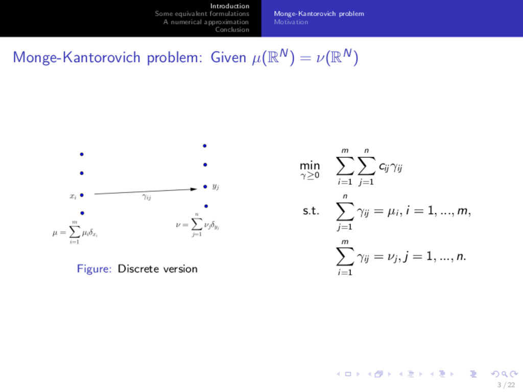
Motivation Monge-Kantorovich problem: Given µ(RN) = ν(RN) Figure: Discrete version min γ≥0 m i=1 n j=1 cij γij s.t. n j=1 γij = µi , i = 1, ..., m, m i=1 γij = νj , j = 1, ..., n. 3 / 22
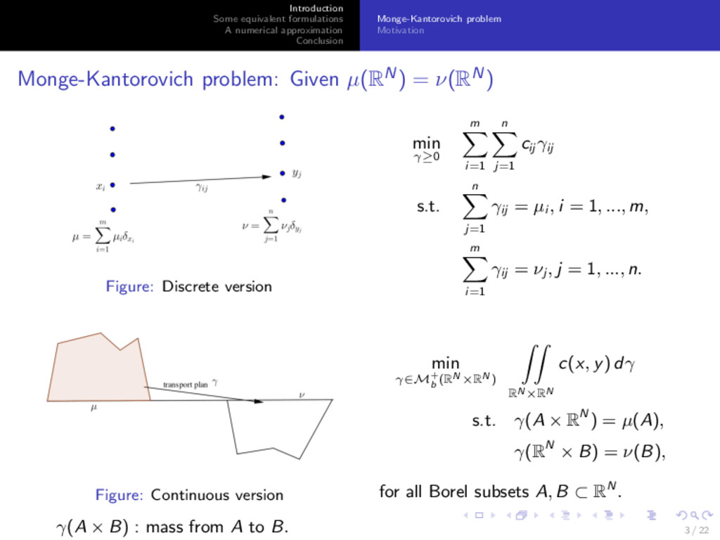
Motivation Monge-Kantorovich problem: Given µ(RN) = ν(RN) Figure: Discrete version min γ≥0 m i=1 n j=1 cij γij s.t. n j=1 γij = µi , i = 1, ..., m, m i=1 γij = νj , j = 1, ..., n. Figure: Continuous version min γ∈M+ b (RN ×RN ) RN ×RN c(x, y) dγ s.t. γ(A × RN ) = µ(A), γ(RN × B) = ν(B), for all Borel subsets A, B ⊂ RN . γ(A × B) : mass from A to B. 3 / 22
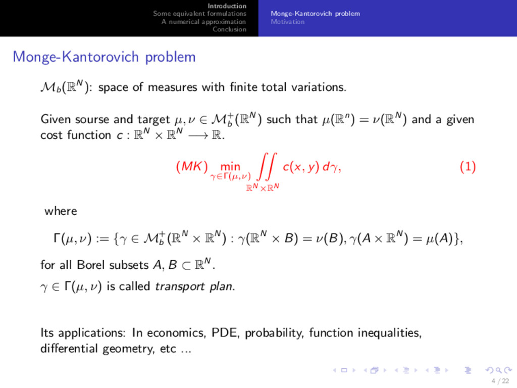
Motivation Monge-Kantorovich problem Mb (RN ): space of measures with finite total variations. Given sourse and target µ, ν ∈ M+ b (RN ) such that µ(Rn) = ν(RN ) and a given cost function c : RN × RN −→ R. (MK) min γ∈Γ(µ,ν) RN ×RN c(x, y) dγ, (1) where Γ(µ, ν) := {γ ∈ M+ b (RN × RN ) : γ(RN × B) = ν(B), γ(A × RN ) = µ(A)}, for all Borel subsets A, B ⊂ RN . γ ∈ Γ(µ, ν) is called transport plan. Its applications: In economics, PDE, probability, function inequalities, differential geometry, etc ... 4 / 22
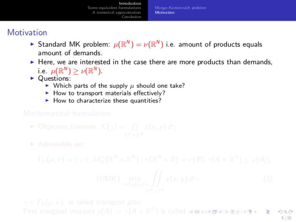
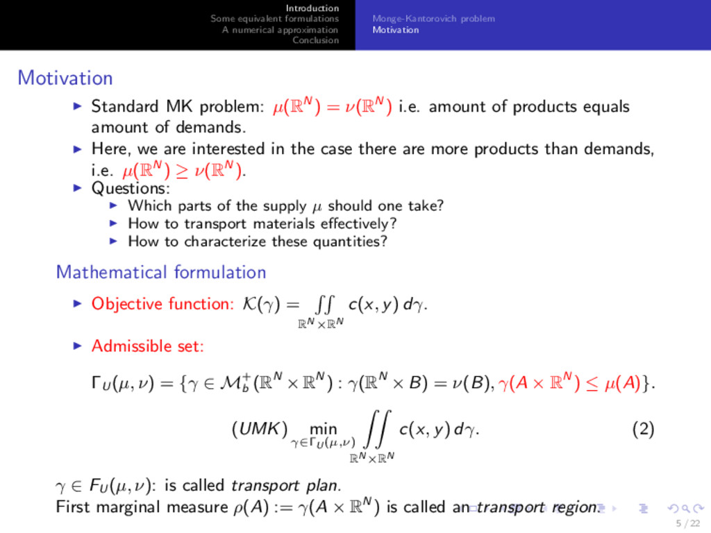
Motivation Motivation Standard MK problem: µ(RN ) = ν(RN ) i.e. amount of products equals amount of demands. Here, we are interested in the case there are more products than demands, i.e. µ(RN ) ≥ ν(RN ). Questions: Which parts of the supply µ should one take? How to transport materials effectively? How to characterize these quantities? Mathematical formulation Objective function: K(γ) = RN ×RN c(x, y) dγ. Admissible set: ΓU (µ, ν) = {γ ∈ M+ b (RN × RN ) : γ(RN × B) = ν(B), γ(A × RN ) ≤ µ(A)}. (UMK) min γ∈ΓU (µ,ν) RN ×RN c(x, y) dγ. (2) γ ∈ FU (µ, ν): is called transport plan. First marginal measure ρ(A) := γ(A × RN ) is called an transport region. 5 / 22
Motivation Motivation Standard MK problem: µ(RN ) = ν(RN ) i.e. amount of products equals amount of demands. Here, we are interested in the case there are more products than demands, i.e. µ(RN ) ≥ ν(RN ). Questions: Which parts of the supply µ should one take? How to transport materials effectively? How to characterize these quantities? Mathematical formulation Objective function: K(γ) = RN ×RN c(x, y) dγ. Admissible set: ΓU (µ, ν) = {γ ∈ M+ b (RN × RN ) : γ(RN × B) = ν(B), γ(A × RN ) ≤ µ(A)}. (UMK) min γ∈ΓU (µ,ν) RN ×RN c(x, y) dγ. (2) γ ∈ FU (µ, ν): is called transport plan. First marginal measure ρ(A) := γ(A × RN ) is called an transport region. 5 / 22
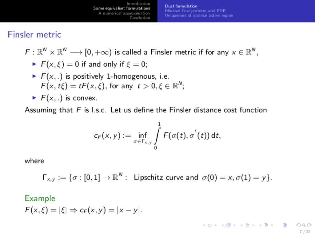
Minimal flow problem and PDE Uniqueness of optimal active region Finsler metric F : RN × RN −→ [0, +∞) is called a Finsler metric if for any x ∈ RN , F(x, ξ) = 0 if and only if ξ = 0; F(x, .) is positively 1-homogenous, i.e. F(x, tξ) = tF(x, ξ), for any t > 0, ξ ∈ RN ; F(x, .) is convex. Assuming that F is l.s.c. Let us define the Finsler distance cost function cF (x, y) := inf σ∈Γx,y 1 0 F(σ(t), σ (t)) dt, where Γx,y := {σ : [0, 1] → RN : Lipschitz curve and σ(0) = x, σ(1) = y}. Example F(x, ξ) = |ξ| ⇒ cF (x, y) = |x − y|. 7 / 22
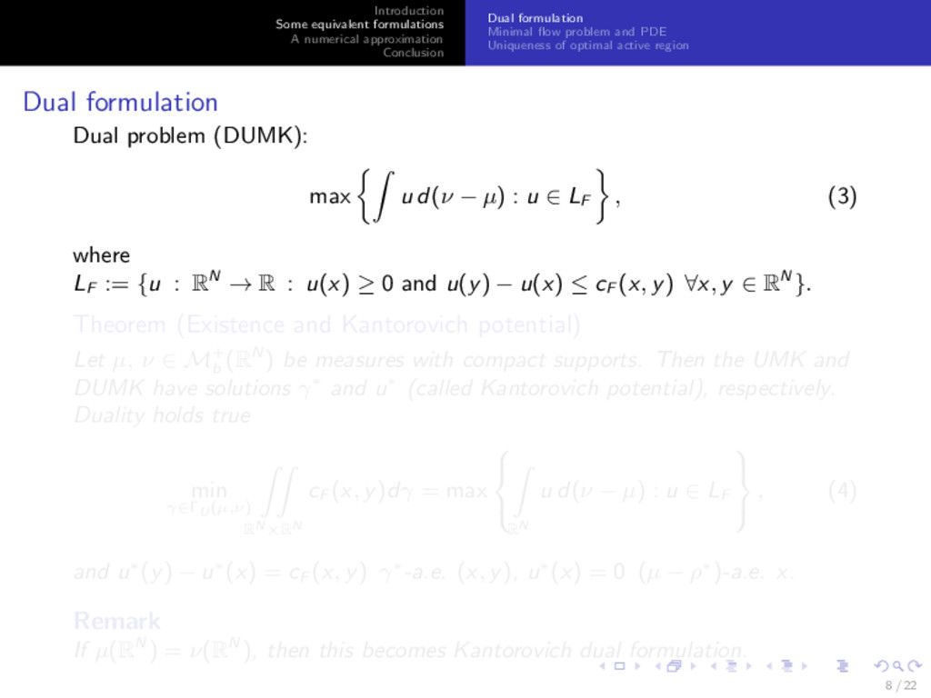
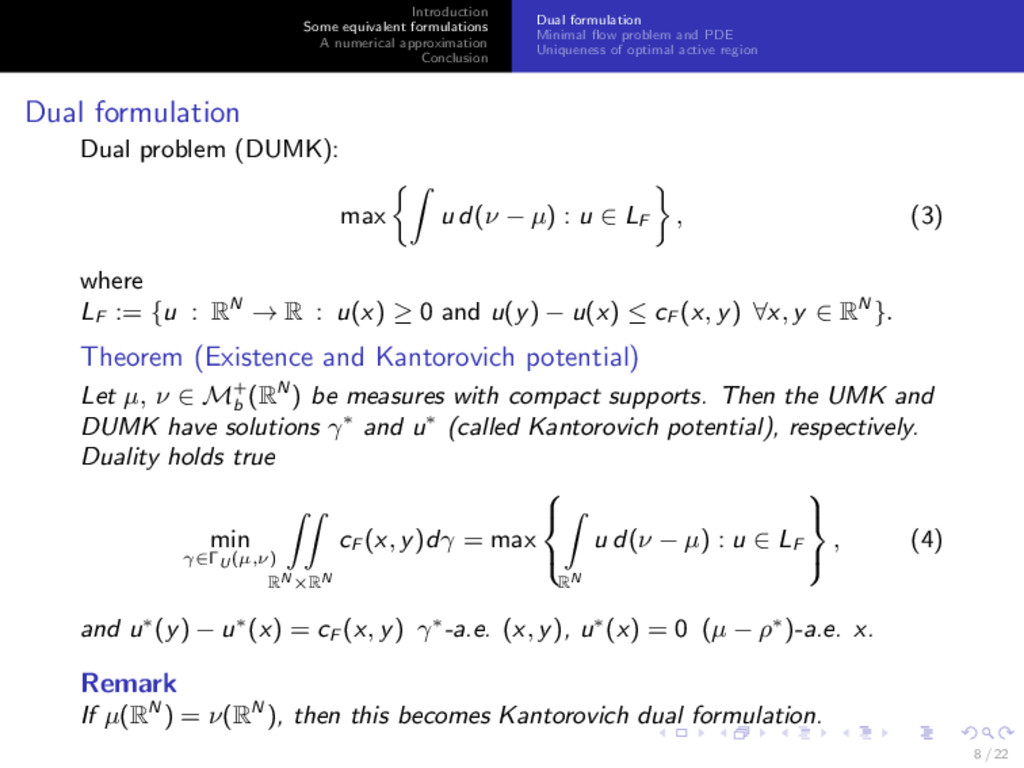
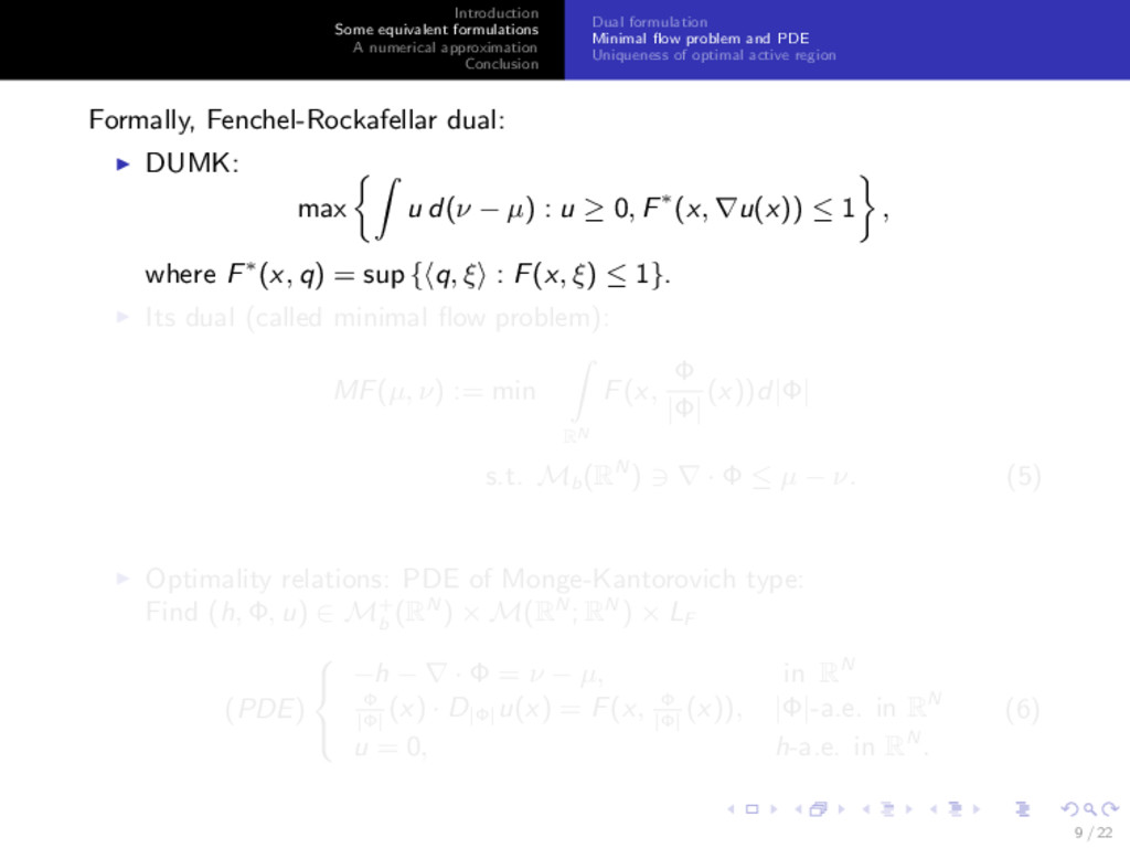
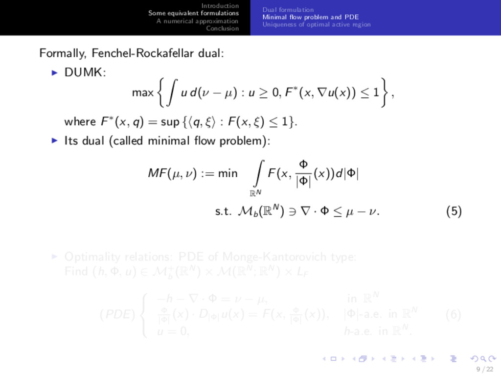
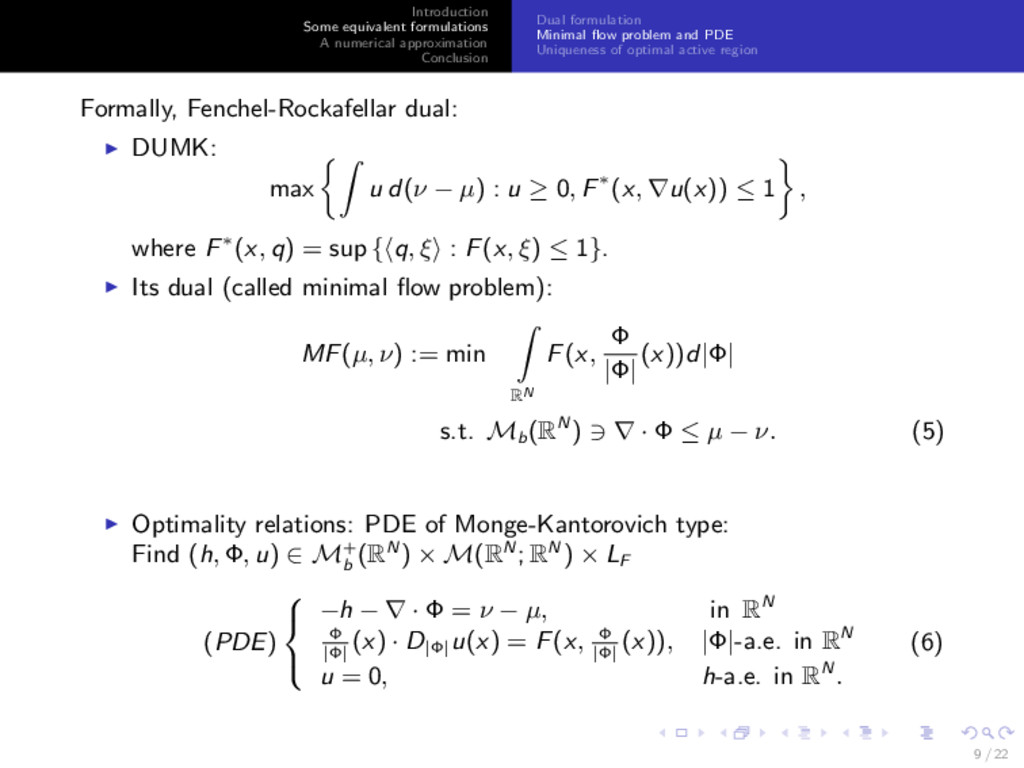
Minimal flow problem and PDE Uniqueness of optimal active region Dual formulation Dual problem (DUMK): max u d(ν − µ) : u ∈ LF , (3) where LF := {u : RN → R : u(x) ≥ 0 and u(y) − u(x) ≤ cF (x, y) ∀x, y ∈ RN }. Theorem (Existence and Kantorovich potential) Let µ, ν ∈ M+ b (RN ) be measures with compact supports. Then the UMK and DUMK have solutions γ∗ and u∗ (called Kantorovich potential), respectively. Duality holds true min γ∈ΓU (µ,ν) RN ×RN cF (x, y)dγ = max RN u d(ν − µ) : u ∈ LF , (4) and u∗(y) − u∗(x) = cF (x, y) γ∗-a.e. (x, y), u∗(x) = 0 (µ − ρ∗)-a.e. x. Remark If µ(RN ) = ν(RN ), then this becomes Kantorovich dual formulation. 8 / 22
Minimal flow problem and PDE Uniqueness of optimal active region Dual formulation Dual problem (DUMK): max u d(ν − µ) : u ∈ LF , (3) where LF := {u : RN → R : u(x) ≥ 0 and u(y) − u(x) ≤ cF (x, y) ∀x, y ∈ RN }. Theorem (Existence and Kantorovich potential) Let µ, ν ∈ M+ b (RN ) be measures with compact supports. Then the UMK and DUMK have solutions γ∗ and u∗ (called Kantorovich potential), respectively. Duality holds true min γ∈ΓU (µ,ν) RN ×RN cF (x, y)dγ = max RN u d(ν − µ) : u ∈ LF , (4) and u∗(y) − u∗(x) = cF (x, y) γ∗-a.e. (x, y), u∗(x) = 0 (µ − ρ∗)-a.e. x. Remark If µ(RN ) = ν(RN ), then this becomes Kantorovich dual formulation. 8 / 22
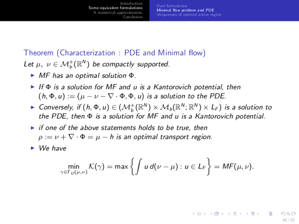
Minimal flow problem and PDE Uniqueness of optimal active region Theorem (Characterization : PDE and Minimal flow) Let µ, ν ∈ M+ b (RN ) be compactly supported. MF has an optimal solution Φ. If Φ is a solution for MF and u is a Kantorovich potential, then (h, Φ, u) := (µ − ν − ∇ · Φ, Φ, u) is a solution to the PDE. Conversely, if (h, Φ, u) ∈ (M+ b (RN ) × Mb (RN ; RN ) × LF ) is a solution to the PDE, then Φ is a solution for MF and u is a Kantorovich potential. if one of the above statements holds to be true, then ρ := ν + ∇ · Φ = µ − h is an optimal transport region. We have min γ∈ΓU (µ,ν) K(γ) = max u d(ν − µ) : u ∈ LF = MF(µ, ν). 10 / 22
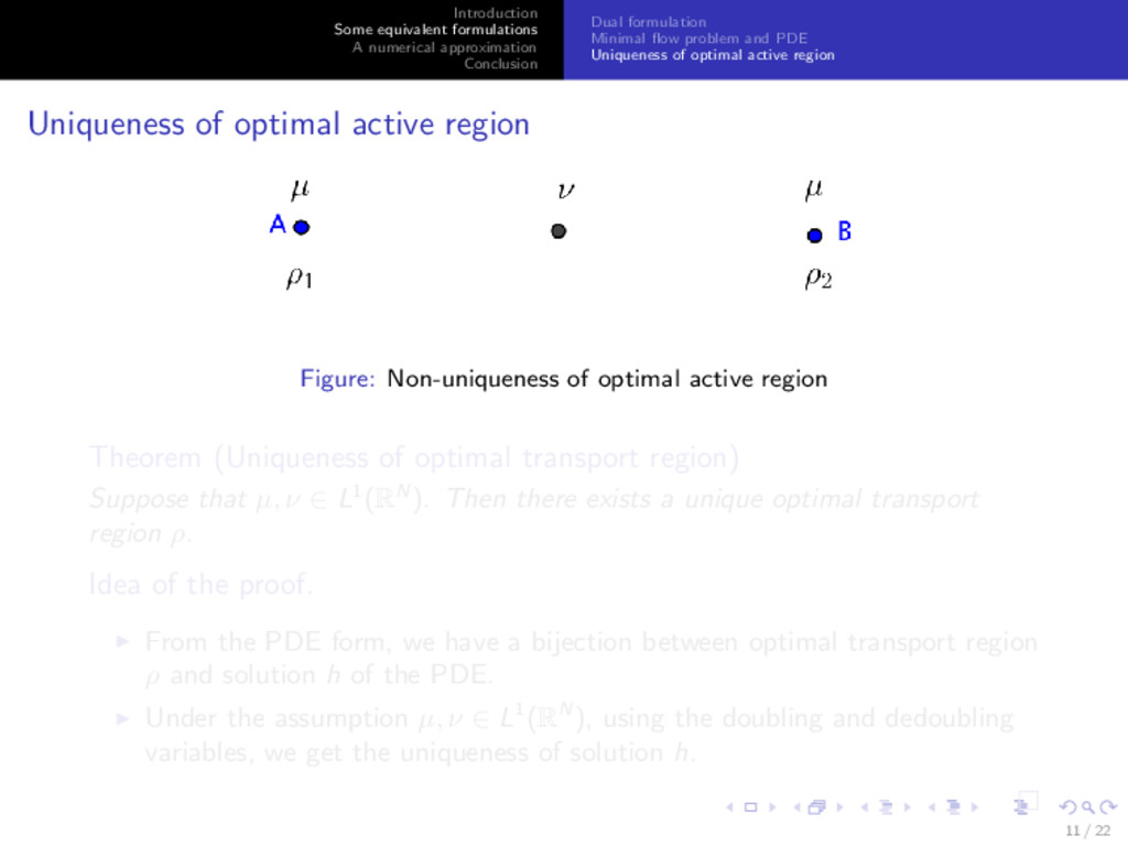
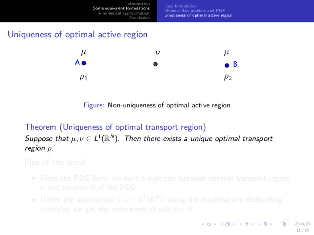
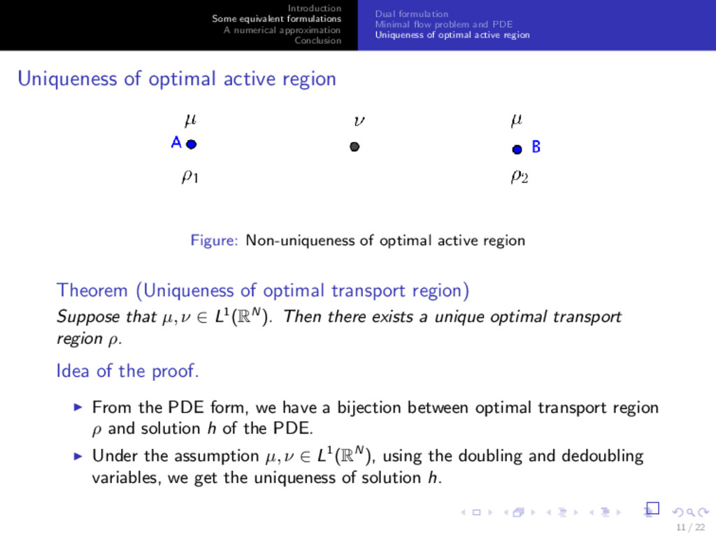
Minimal flow problem and PDE Uniqueness of optimal active region Uniqueness of optimal active region Figure: Non-uniqueness of optimal active region Theorem (Uniqueness of optimal transport region) Suppose that µ, ν ∈ L1(RN ). Then there exists a unique optimal transport region ρ. Idea of the proof. From the PDE form, we have a bijection between optimal transport region ρ and solution h of the PDE. Under the assumption µ, ν ∈ L1(RN ), using the doubling and dedoubling variables, we get the uniqueness of solution h. 11 / 22
Minimal flow problem and PDE Uniqueness of optimal active region Uniqueness of optimal active region Figure: Non-uniqueness of optimal active region Theorem (Uniqueness of optimal transport region) Suppose that µ, ν ∈ L1(RN ). Then there exists a unique optimal transport region ρ. Idea of the proof. From the PDE form, we have a bijection between optimal transport region ρ and solution h of the PDE. Under the assumption µ, ν ∈ L1(RN ), using the doubling and dedoubling variables, we get the uniqueness of solution h. 11 / 22
Minimal flow problem and PDE Uniqueness of optimal active region Uniqueness of optimal active region Figure: Non-uniqueness of optimal active region Theorem (Uniqueness of optimal transport region) Suppose that µ, ν ∈ L1(RN ). Then there exists a unique optimal transport region ρ. Idea of the proof. From the PDE form, we have a bijection between optimal transport region ρ and solution h of the PDE. Under the assumption µ, ν ∈ L1(RN ), using the doubling and dedoubling variables, we get the uniqueness of solution h. 11 / 22
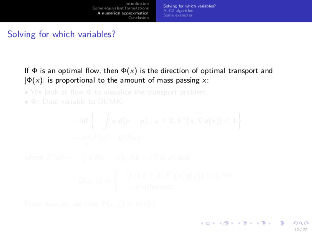
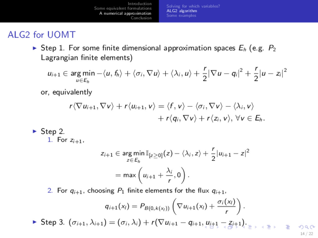
which variables? ALG2 algorithm Some examples Solving for which variables? If Φ is an optimal flow, then Φ(x) is the direction of optimal transport and |Φ(x)| is proportional to the amount of mass passing x: • We look at flow Φ to visualize the transport problem. • Φ: Dual variable to DUMK: − inf − u d(ν − µ) : u ≥ 0, F∗(x, ∇u(x)) ≤ 1 inf u F(u) + G(Λu), where F(u) = − u d(ν − µ), Λu = (∇u, u) and G(q, z) = 0 if z ≥ 0, F∗(x, q(x)) ≤ 1, ∀x +∞ otherwise. From now on, we take F(x, ξ) = k(x)|ξ|. 12 / 22
which variables? ALG2 algorithm Some examples Solving for which variables? If Φ is an optimal flow, then Φ(x) is the direction of optimal transport and |Φ(x)| is proportional to the amount of mass passing x: • We look at flow Φ to visualize the transport problem. • Φ: Dual variable to DUMK: − inf − u d(ν − µ) : u ≥ 0, F∗(x, ∇u(x)) ≤ 1 inf u F(u) + G(Λu), where F(u) = − u d(ν − µ), Λu = (∇u, u) and G(q, z) = 0 if z ≥ 0, F∗(x, q(x)) ≤ 1, ∀x +∞ otherwise. From now on, we take F(x, ξ) = k(x)|ξ|. 12 / 22
which variables? ALG2 algorithm Some examples Solving for which variables? If Φ is an optimal flow, then Φ(x) is the direction of optimal transport and |Φ(x)| is proportional to the amount of mass passing x: • We look at flow Φ to visualize the transport problem. • Φ: Dual variable to DUMK: − inf − u d(ν − µ) : u ≥ 0, F∗(x, ∇u(x)) ≤ 1 inf u F(u) + G(Λu), where F(u) = − u d(ν − µ), Λu = (∇u, u) and G(q, z) = 0 if z ≥ 0, F∗(x, q(x)) ≤ 1, ∀x +∞ otherwise. From now on, we take F(x, ξ) = k(x)|ξ|. 12 / 22
which variables? ALG2 algorithm Some examples Solving for which variables? If Φ is an optimal flow, then Φ(x) is the direction of optimal transport and |Φ(x)| is proportional to the amount of mass passing x: • We look at flow Φ to visualize the transport problem. • Φ: Dual variable to DUMK: − inf − u d(ν − µ) : u ≥ 0, F∗(x, ∇u(x)) ≤ 1 inf u F(u) + G(Λu), where F(u) = − u d(ν − µ), Λu = (∇u, u) and G(q, z) = 0 if z ≥ 0, F∗(x, q(x)) ≤ 1, ∀x +∞ otherwise. From now on, we take F(x, ξ) = k(x)|ξ|. 12 / 22
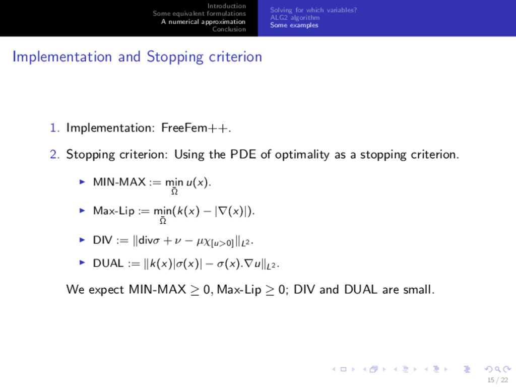
which variables? ALG2 algorithm Some examples Implementation and Stopping criterion 1. Implementation: FreeFem++. 2. Stopping criterion: Using the PDE of optimality as a stopping criterion. MIN-MAX := min ¯ Ω u(x). Max-Lip := min ¯ Ω (k(x) − |∇(x)|). DIV := divσ + ν − µχ[u>0] L2 . DUAL := k(x)|σ(x)| − σ(x).∇u L2 . We expect MIN-MAX ≥ 0, Max-Lip ≥ 0; DIV and DUAL are small. 15 / 22
which variables? ALG2 algorithm Some examples Implementation and Stopping criterion 1. Implementation: FreeFem++. 2. Stopping criterion: Using the PDE of optimality as a stopping criterion. MIN-MAX := min ¯ Ω u(x). Max-Lip := min ¯ Ω (k(x) − |∇(x)|). DIV := divσ + ν − µχ[u>0] L2 . DUAL := k(x)|σ(x)| − σ(x).∇u L2 . We expect MIN-MAX ≥ 0, Max-Lip ≥ 0; DIV and DUAL are small. 15 / 22
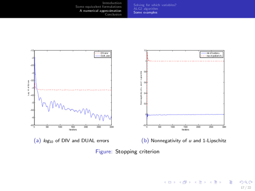
which variables? ALG2 algorithm Some examples 0 500 1000 1500 2000 2500 3000 −6.5 −6 −5.5 −5 −4.5 −4 −3.5 −3 −2.5 −2 −1.5 Iterations Log 10 of Errors DIV error DUAL error (a) log10 of DIV and DUAL errors 0 500 1000 1500 2000 2500 3000 −0.2 0 0.2 0.4 0.6 0.8 1 1.2 Iterations Nonnegativity of u, and 1−Lipschitz min of function u max of gradient of u (b) Nonnegativity of u and 1-Lipschitz Figure: Stopping criterion 17 / 22
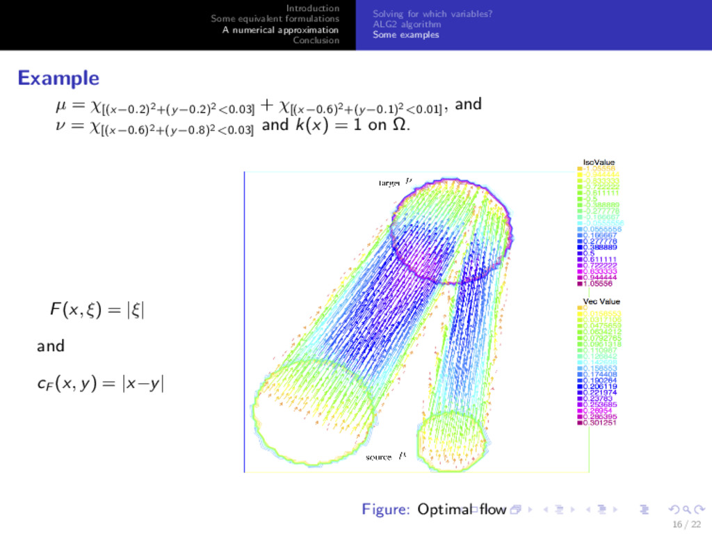
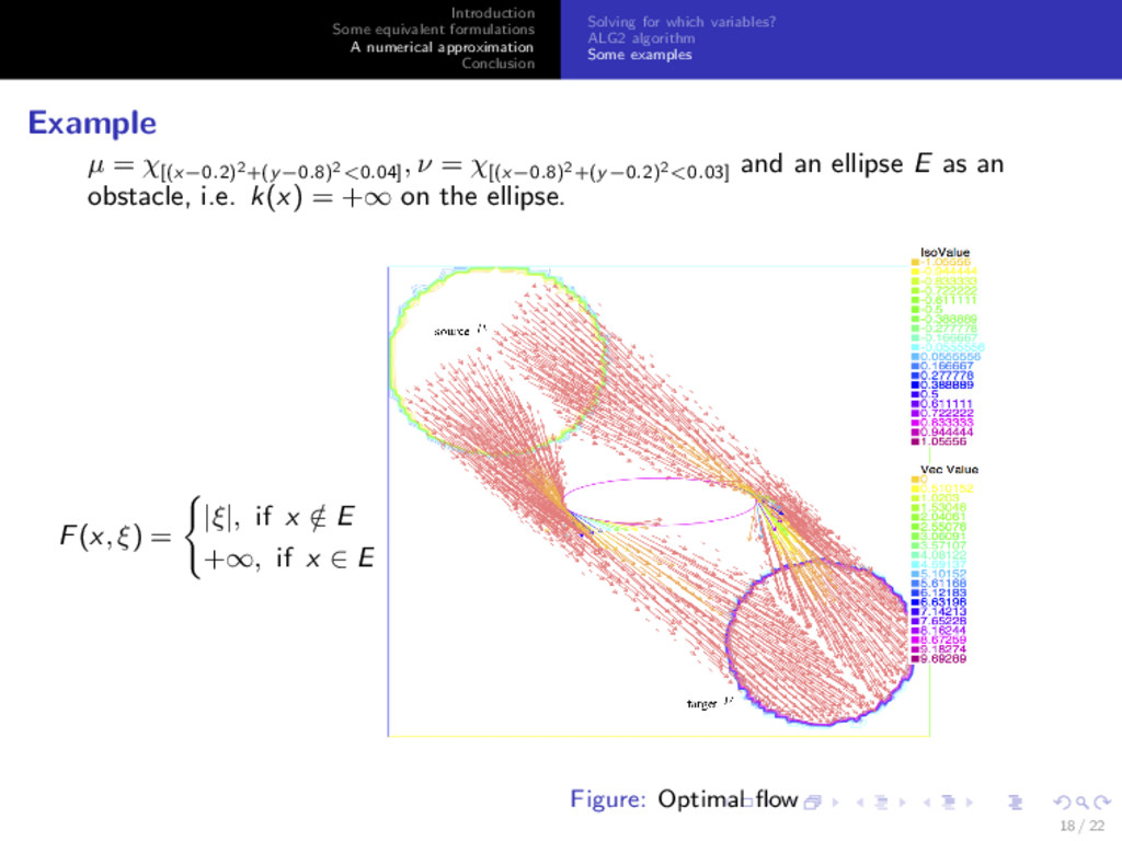
which variables? ALG2 algorithm Some examples Example µ = χ[(x−0.2)2+(y−0.8)2<0.04] , ν = χ[(x−0.8)2+(y−0.2)2<0.03] and an ellipse E as an obstacle, i.e. k(x) = +∞ on the ellipse. F(x, ξ) = |ξ|, if x / ∈ E +∞, if x ∈ E. Figure: Optimal flow 18 / 22
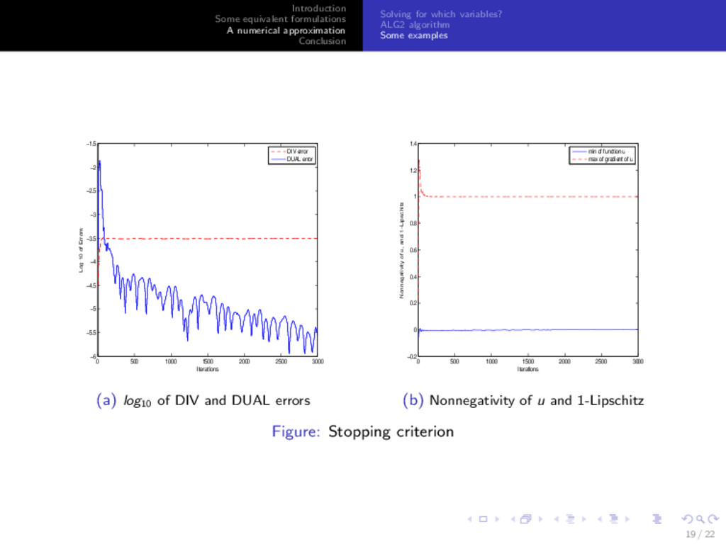
which variables? ALG2 algorithm Some examples 0 500 1000 1500 2000 2500 3000 −6 −5.5 −5 −4.5 −4 −3.5 −3 −2.5 −2 −1.5 Iterations Log 10 of Errors DIV error DUAL error (a) log10 of DIV and DUAL errors 0 500 1000 1500 2000 2500 3000 −0.2 0 0.2 0.4 0.6 0.8 1 1.2 1.4 Iterations Nonnegativity of u, and 1−Lipschitz min of function u max of gradient of u (b) Nonnegativity of u and 1-Lipschitz Figure: Stopping criterion 19 / 22
Introducing some equivalent formulations for unbalanced optimal transport: Dual formulation Minimal flow PDE of optimality relations 2. Showing the uniqueness of optimal active region under some conditions. 3. Using above formulations to give a numerical approximation. 20 / 22
Ambrosio. Lecture notes on optimal transport problems. Springer, Berlin, 2003. J. W. Barrett and L. Prigozhin. Partial L1 Monge-Kantorovich problem: Variational formulation and numerical approximation. Interfaces and Free Boundaries, 11(2), (2009), 201-238. L. A. Caffarelli and R. J. McCann. Free boundaries in optimal transport and Monge-Amp` ere obstacle problems. Annals of Mathematics. 171, (2010), 673–730. J. Eckstein and D. P. Bertsekas. On the Douglas–Rachford splitting method and the proximal point algorithm for maximal monotone operators. Mathematical Programming 55.1-3 (1992): 293-318. C. Villani. Optimal Transport, Old and New, Grundlehren des Mathematischen Wissenschaften (Fundamental Principles of Mathematical Sciences), Vol. 338, Springer-Verlag, Berlin-New York, 2009. 21 / 22