Theoretical study of steerable homogeneous operators

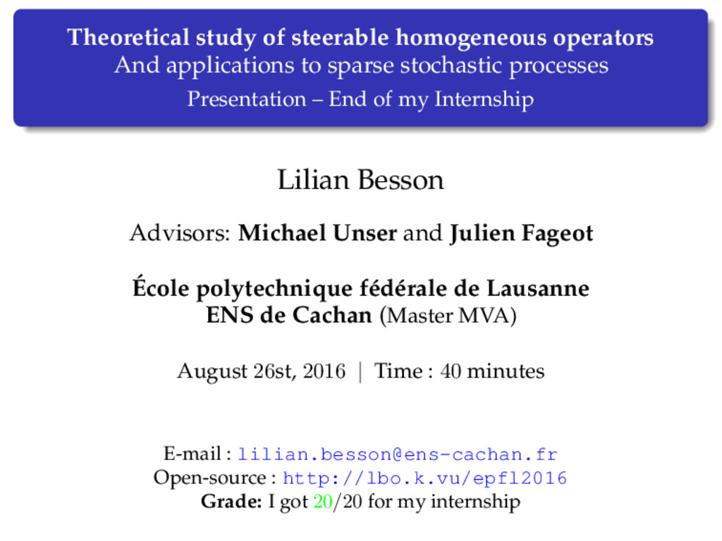
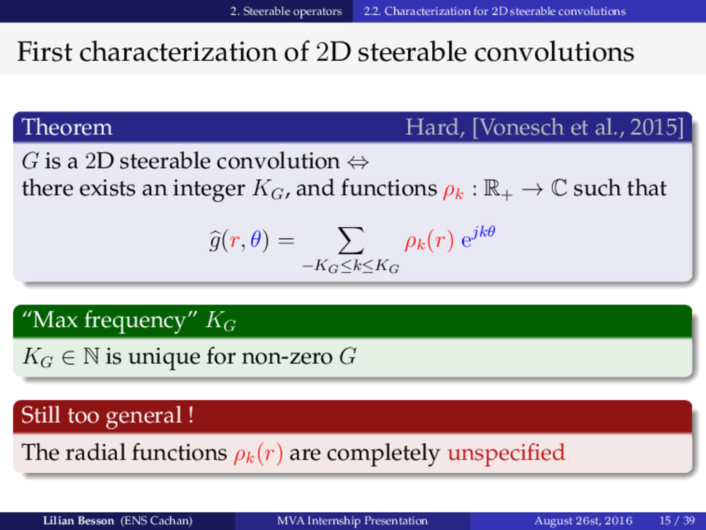
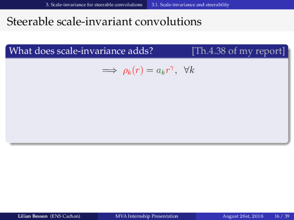
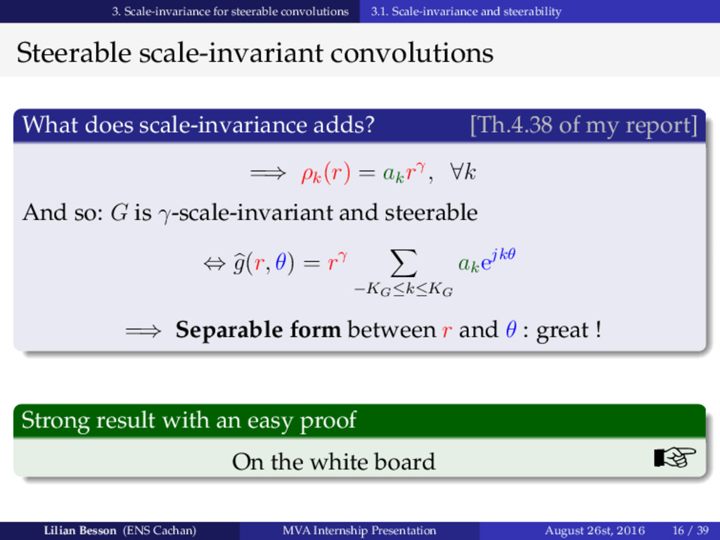
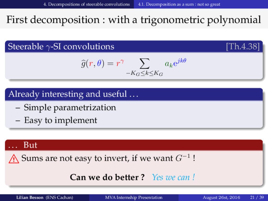
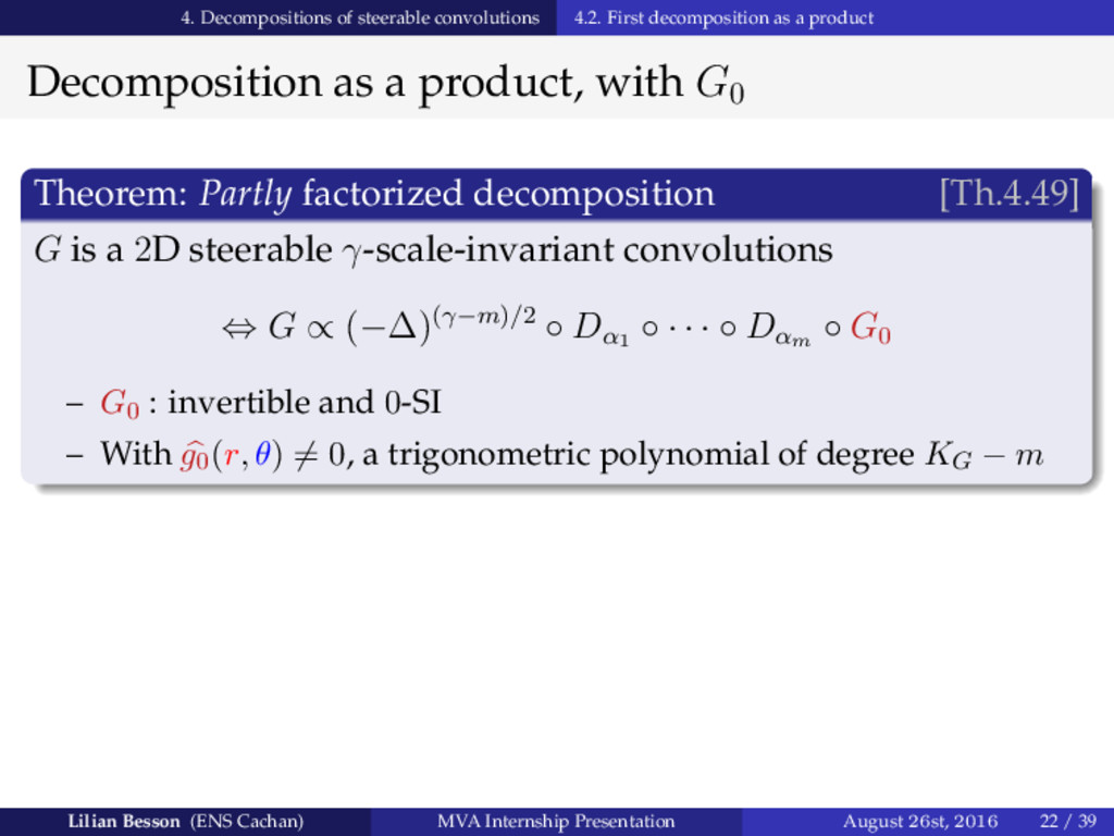
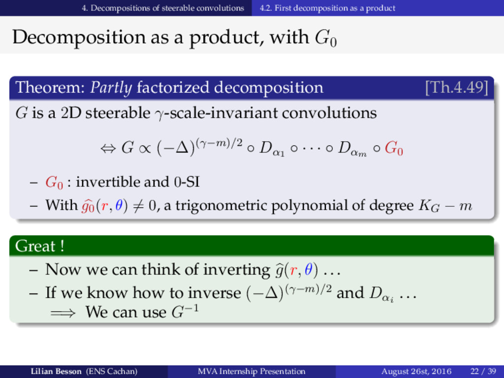
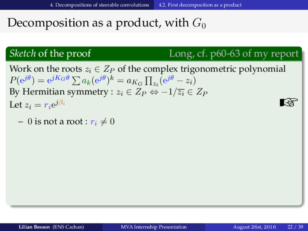
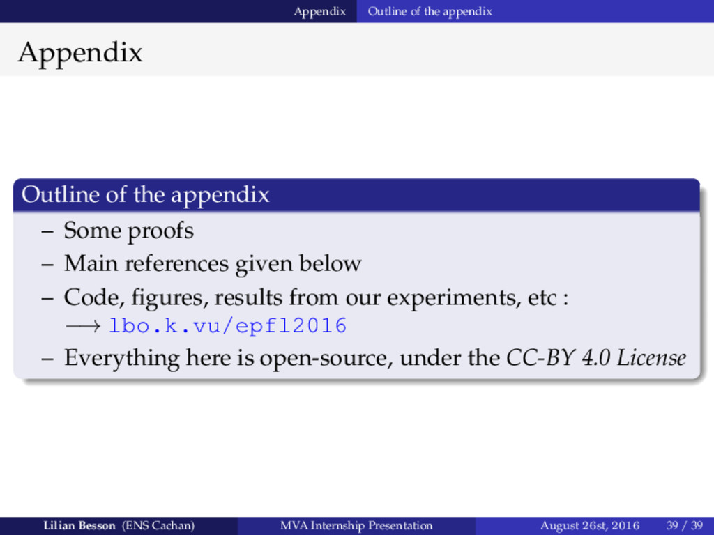
Theoretical study of steerable homogeneous operators and applications to sparse stochastic processes.

Slides in English for my oral presentation at the end of my Masters of Science research internship.
5 months internship in Lausanne, Switzerland, at EPFL in the BIG team, under the supervision of Julien Fageot and Michael Unser.

PDF: https://perso.crans.org/besson/slidesM2MVA16.pdf

Transcript

1. Theoretical study of steerable homogeneous operators And applications to sparse stochastic processes Presentation – End of my Internship Lilian Besson Advisors: Michael Unser and Julien Fageot École polytechnique fédérale de Lausanne ENS de Cachan (Master MVA) August 26st, 2016 | Time : 40 minutes E-mail : lilian.besson@ens-cachan.fr Open-source : http://lbo.k.vu/epfl2016 Grade: I got 20/20 for my internship
2. Introduction & Motivations 0.1. Subject of my internship Subject Functional operators Mainly about convolution operators (= linear + continuous + translation-invariant, “LSI”) Steerable and homogeneous convolutions – More freedom than if rotation-invariant – But still easily parametrized ! Lilian Besson (ENS Cachan) MVA Internship Presentation August 26st, 2016 1 / 39
3. Introduction & Motivations 0.1. Subject of my internship Subject Functional operators Mainly about convolution operators (= linear + continuous + translation-invariant, “LSI”) Steerable and homogeneous convolutions – More freedom than if rotation-invariant – But still easily parametrized ! Applications and experiments Mainly on sparse stochastic processes, in 2D Lilian Besson (ENS Cachan) MVA Internship Presentation August 26st, 2016 1 / 39
4. Introduction & Motivations 0.2. Motivations Apply our operators to ... Sparse processes [Unser and Tafti, 2014] – To visualize their effects – To generate new processes – . . . and see pretty images ! Lilian Besson (ENS Cachan) MVA Internship Presentation August 26st, 2016 2 / 39
5. Introduction & Motivations 0.2. Motivations Apply our operators to ... Sparse processes [Unser and Tafti, 2014] – To visualize their effects – To generate new processes – . . . and see pretty images ! Splines [Unser et al., 2016] – One operator ⇐⇒ one spline Lilian Besson (ENS Cachan) MVA Internship Presentation August 26st, 2016 2 / 39
6. Introduction & Motivations 0.3. Outline Outline 1 Reminders on operators theory 2 Steerable operators 3 Scale-invariance for steerable convolutions 4 Decompositions of steerable convolutions 5 Illustrations on sparse stochastic processes 6 Conclusion & Appendix Lilian Besson (ENS Cachan) MVA Internship Presentation August 26st, 2016 3 / 39
7. 1. Reminders on operators theory 1 Reminders on operators theory Lilian Besson (ENS Cachan) MVA Internship Presentation August 26st, 2016 4 / 39
8. 1. Reminders on operators theory 1.1. Reminders on operators What are operators ? An operator Takes a function , transforms it to another function {} For real-valued , has to give a real-valued {} Lilian Besson (ENS Cachan) MVA Internship Presentation August 26st, 2016 4 / 39
9. 1. Reminders on operators theory 1.1. Reminders on operators What are operators ? An operator Takes a function , transforms it to another function {} For real-valued , has to give a real-valued {} Examples in maths – Derivatives and , Laplacian Δ – Denoising, contour detection, etc Examples in real life ? – “Filters” for photos, in Instagram or Facebook ! – Rotating photos, etc Lilian Besson (ENS Cachan) MVA Internship Presentation August 26st, 2016 4 / 39
10. 1. Reminders on operators theory 1.1. Reminders on operators Different properties for operators Today, our operators are always – Linear – Continuous – In 2D : : (, ) ↦→ {}(, ) – Translation-invariance Lilian Besson (ENS Cachan) MVA Internship Presentation August 26st, 2016 5 / 39
11. 1. Reminders on operators theory 1.1. Reminders on operators Different properties for operators Today, our operators are always – Linear – Continuous – In 2D : : (, ) ↦→ {}(, ) – Translation-invariance Geometric properties [Unser and Tafti, 2014] – Scale-invariance or -scale-invariance (= homogeneity) – Rotation-invariance – Steerable Lilian Besson (ENS Cachan) MVA Internship Presentation August 26st, 2016 5 / 39
12. 1. Reminders on operators theory 1.2. Schwartz theorem for convolution operators Schwartz theorem and impulse response Schwartz convolution theorem [Stein and Weiss, 1971] Translation-invariant linear continuous operators are exactly convolution operators : {} = ( * ) Lilian Besson (ENS Cachan) MVA Internship Presentation August 26st, 2016 6 / 39
13. 1. Reminders on operators theory 1.2. Schwartz theorem for convolution operators Schwartz theorem and impulse response Schwartz convolution theorem [Stein and Weiss, 1971] Translation-invariant linear continuous operators are exactly convolution operators : {} = ( * ) Impulse response of = {0 } is a distribution (= generalized function) Lilian Besson (ENS Cachan) MVA Internship Presentation August 26st, 2016 6 / 39
14. 1. Reminders on operators theory 1.2. Schwartz theorem for convolution operators Fourier multiplier ̂︀ of an operator Using the Fourier transform ℱ [Stein and Weiss, 1971] ℱ transforms a convolution ( * ) to a point-wise product So ℱ{︁{}}︁ = ℱ{ * } = ℱ{} · ℱ{} = ̂︀ · ̂︀ Fourier multiplier ̂︀ And so {} = ℱ−1{︁ ̂︀ · ̂︀ }︁ ̂︀ = ℱ{} is a complex-valued function Lilian Besson (ENS Cachan) MVA Internship Presentation August 26st, 2016 7 / 39
15. 1. Reminders on operators theory 1.2. Schwartz theorem for convolution operators Using the Fourier multiplier ̂︀ Working in the “Fourier domain” Output function {}(, ) Output in Fourier ̂︀ (, ) · ̂︀ (, ) Input in Fourier ̂︀ (, ) Input function (, ) ℱ Point-wise multiplication by ̂︀ (, ) ℱ−1 In 2D, the Fourier variable is written in polar coordinates : = (, ) Lilian Besson (ENS Cachan) MVA Internship Presentation August 26st, 2016 8 / 39
16. 1. Reminders on operators theory 1.3. Geometric properties and characterizations Property: scale-invariance Definition For > 0, is -scale-invariant when {}( [︃/ / ]︃ ) = {(·/)}( [︃ ]︃ ), ∀ scaling > 0 Lilian Besson (ENS Cachan) MVA Internship Presentation August 26st, 2016 9 / 39
17. 1. Reminders on operators theory 1.3. Geometric properties and characterizations Property: scale-invariance Definition For > 0, is -scale-invariant when {}( [︃/ / ]︃ ) = {(·/)}( [︃ ]︃ ), ∀ scaling > 0 Easy characterization on ̂︀ ̂︀ (, ) = ̂︀ (, ), ∀ > 0 Separable form for ̂︀ – ̂︀ (, ) = ̂︀ (1, ) – ̂︀ (1, ) only depends on the angle Lilian Besson (ENS Cachan) MVA Internship Presentation August 26st, 2016 9 / 39
18. 1. Reminders on operators theory 1.3. Geometric properties and characterizations Example #1: derivatives Derivatives and directional derivatives – Usual derivatives : and – Directional derivative : def = cos() + sin() They are 1-scale-invariant Because their Fourier multipliers are – ̂︂ (, ) = = cos() – ̂︂ (, ) = = sin() – ̂︂ (, ) = cos( − ) Lilian Besson (ENS Cachan) MVA Internship Presentation August 26st, 2016 10 / 39
19. 1. Reminders on operators theory 1.3. Geometric properties and characterizations Property: rotation-invariance Definition is rotation-invariant when {}(0 [︃ ]︃ ) = {(0 ·)}( [︃ ]︃ ) ∀ rotation 0 Lilian Besson (ENS Cachan) MVA Internship Presentation August 26st, 2016 11 / 39
20. 1. Reminders on operators theory 1.3. Geometric properties and characterizations Property: rotation-invariance Definition is rotation-invariant when {}(0 [︃ ]︃ ) = {(0 ·)}( [︃ ]︃ ) ∀ rotation 0 Easy characterization on ̂︀ ̂︀ (, + 0 ) = ̂︀ (, ), ∀ rotation angle 0 Purely radial ̂︀ ̂︀ (, ) = ̂︀ (, 0) only depends on the radius : ̂︀ is purely radial ! Lilian Besson (ENS Cachan) MVA Internship Presentation August 26st, 2016 11 / 39
21. 1. Reminders on operators theory 1.3. Geometric properties and characterizations Example #2: fractional Laplacians Laplacian and fractional Laplacians [Unser and Tafti, 2014] For > 0, (−Δ)/2 has a Fourier multiplier ̂︀ (, ) = So they are ... – -scale-invariant – and rotation-invariant =⇒ Simplest example of -SI and RI operators ! In fact . . . Lilian Besson (ENS Cachan) MVA Internship Presentation August 26st, 2016 12 / 39
22. 1. Reminders on operators theory 1.3. Geometric properties and characterizations Example #2: fractional Laplacians Laplacian and fractional Laplacians [Unser and Tafti, 2014] For > 0, (−Δ)/2 has a Fourier multiplier ̂︀ (, ) = So they are ... – -scale-invariant – and rotation-invariant =⇒ Simplest example of -SI and RI operators ! Theorem: -SI + RI ⇔ Laplacian [Th.3.39 of my report] (−Δ)/2 is the only -SI and RI convolution Lilian Besson (ENS Cachan) MVA Internship Presentation August 26st, 2016 12 / 39
23. 2. Steerable operators 2 Steerable operators Lilian Besson (ENS Cachan) MVA Internship Presentation August 26st, 2016 13 / 39
24. 2. Steerable operators 2.1. Definition of steerability Steerable convolution operators Definition [Vonesch et al., 2015],[Unser and Chenouard, 2013] is steerable when dim ^ = dim Span 0∈[0,2] {︁(, ) ↦→ ̂︀ (, + 0 )}︁ is finite Lilian Besson (ENS Cachan) MVA Internship Presentation August 26st, 2016 13 / 39
25. 2. Steerable operators 2.1. Definition of steerability Steerable convolution operators Definition [Vonesch et al., 2015],[Unser and Chenouard, 2013] is steerable when dim ^ = dim Span 0∈[0,2] {︁(, ) ↦→ ̂︀ (, + 0 )}︁ is finite Order of steerability def = dim ^ ∈ N Example: Null-operator = 0 ⇔ = 0 Lilian Besson (ENS Cachan) MVA Internship Presentation August 26st, 2016 13 / 39
26. 2. Steerable operators 2.1. Definition of steerability Steerability generalizes rotation-invariance Theorem [Th.4.22 of my report] Non-zero steerable of order = 1 ⇔ rotation-invariant Just a sanity check ... Lilian Besson (ENS Cachan) MVA Internship Presentation August 26st, 2016 14 / 39
27. 2. Steerable operators 2.2. Characterization for 2D steerable convolutions First characterization of 2D steerable convolutions Theorem Hard, [Vonesch et al., 2015] is a 2D steerable convolution ⇔ there exists an integer , and functions : R+ → C such that ̂︀ (, ) = ∑︁ −≤≤ () e Lilian Besson (ENS Cachan) MVA Internship Presentation August 26st, 2016 15 / 39
28. 2. Steerable operators 2.2. Characterization for 2D steerable convolutions First characterization of 2D steerable convolutions Theorem Hard, [Vonesch et al., 2015] is a 2D steerable convolution ⇔ there exists an integer , and functions : R+ → C such that ̂︀ (, ) = ∑︁ −≤≤ () e “Max frequency” ∈ N is unique for non-zero Lilian Besson (ENS Cachan) MVA Internship Presentation August 26st, 2016 15 / 39
29. 2. Steerable operators 2.2. Characterization for 2D steerable convolutions First characterization of 2D steerable convolutions Theorem Hard, [Vonesch et al., 2015] is a 2D steerable convolution ⇔ there exists an integer , and functions : R+ → C such that ̂︀ (, ) = ∑︁ −≤≤ () e “Max frequency” ∈ N is unique for non-zero Still too general ! The radial functions () are completely unspecified Lilian Besson (ENS Cachan) MVA Internship Presentation August 26st, 2016 15 / 39
30. 3. Scale-invariance for steerable convolutions 3 Scale-invariance for steerable convolutions Lilian Besson (ENS Cachan) MVA Internship Presentation August 26st, 2016 16 / 39
31. 3. Scale-invariance for steerable convolutions 3.1. Scale-invariance and steerability Steerable scale-invariant convolutions What does scale-invariance adds? [Th.4.38 of my report] =⇒ () = , ∀ Lilian Besson (ENS Cachan) MVA Internship Presentation August 26st, 2016 16 / 39
32. 3. Scale-invariance for steerable convolutions 3.1. Scale-invariance and steerability Steerable scale-invariant convolutions What does scale-invariance adds? [Th.4.38 of my report] =⇒ () = , ∀ And so: is -scale-invariant and steerable ⇔ ̂︀ (, ) = ∑︁ −≤≤ e =⇒ Separable form between and : great ! Strong result with an easy proof On the white board Lilian Besson (ENS Cachan) MVA Internship Presentation August 26st, 2016 16 / 39
33. 3. Scale-invariance for steerable convolutions 3.1. Scale-invariance and steerability Steerable scale-invariant convolutions What does scale-invariance adds? [Th.4.38 of my report] =⇒ () = , ∀ And so: is -scale-invariant and steerable ⇔ ̂︀ (, ) = ∑︁ −≤≤ e =⇒ Separable form between and : great ! Parametrization of steerable -SI convolutions new ! With ∈ N and 2 + 1 complex parameters = (1) And their polar part is just a trigonometric polynomial (in e) ! Lilian Besson (ENS Cachan) MVA Internship Presentation August 26st, 2016 16 / 39
34. 3. Scale-invariance for steerable convolutions 3.2. And for real convolution operators ? Hermitian-symmetric Fourier multiplier Hermitian-symmetric ̂︀ [Stein and Weiss, 1971] is real ⇔ ∀, {} is real-valued ⇔ ̂︀ is Hermitian-symmetric : ̂︀ (, + ) = ̂︀ (, ) Lilian Besson (ENS Cachan) MVA Internship Presentation August 26st, 2016 17 / 39
35. 3. Scale-invariance for steerable convolutions 3.2. And for real convolution operators ? Hermitian-symmetric Fourier multiplier Hermitian-symmetric ̂︀ [Stein and Weiss, 1971] is real ⇔ ∀, {} is real-valued ⇔ ̂︀ is Hermitian-symmetric : ̂︀ (, + ) = ̂︀ (, ) Consequence on the coefficients ( ) ? − = (−1) , ∀ Parametrization better ! =⇒ With ∈ N and parameters {0, . . . , } only Lilian Besson (ENS Cachan) MVA Internship Presentation August 26st, 2016 17 / 39
36. 3. Scale-invariance for steerable convolutions 3.3. Important examples: differential operators Example with = 1 : the fractional Laplacian = (−Δ)/2 is steerable, of order = 1 Fourier multiplier ̂︀ (, ) = is Hermitian-symmetric, RI and -SI With our parametrization With = 0, and 0 = 1 Check: 0 = (−1)00 Lilian Besson (ENS Cachan) MVA Internship Presentation August 26st, 2016 18 / 39
37. 3. Scale-invariance for steerable convolutions 3.3. Important examples: differential operators Example with = 2 : directional derivatives = is steerable, of order = 2 Fourier multiplier [Chaudhury and Unser, 2010] ̂︀ (, ) = cos( − ) is Hermitian-symmetric, not RI and 1-SI With our parametrization With = 1, and −1 = e−/2, 0 = 0, 1 = e/2 Check: −1 = (−1)11 Lilian Besson (ENS Cachan) MVA Internship Presentation August 26st, 2016 19 / 39
38. 3. Scale-invariance for steerable convolutions 3.3. Important examples: differential operators Example with = 2 : directional derivatives = is steerable, of order = 2 Fourier multiplier [Chaudhury and Unser, 2010] ̂︀ (, ) = cos( − ) is Hermitian-symmetric, not RI and 1-SI Sanity check And it has = 2 Good: steerability is more general than rotation-invariant Lilian Besson (ENS Cachan) MVA Internship Presentation August 26st, 2016 19 / 39
39. 3. Scale-invariance for steerable convolutions 3.3. Important examples: differential operators Example with = 3 : the “Mondrian” = is steerable, of order = 3 Fourier multiplier ̂︀ (, ) = −2 cos() sin() is Hermitian-sym., not RI and 2-SI With our parametrization With = 2, and −2 = −/4, −1 = 0 = 1 = 0, 2 = /4 Check: −2 = (−1)22 Lilian Besson (ENS Cachan) MVA Internship Presentation August 26st, 2016 20 / 39
40. 4. Decompositions of steerable convolutions 4 Decompositions of steerable convolutions Lilian Besson (ENS Cachan) MVA Internship Presentation August 26st, 2016 21 / 39
41. 4. Decompositions of steerable convolutions 4.1. Decomposition as a sum : not so great First decomposition : with a trigonometric polynomial Steerable -SI convolutions [Th.4.38] ̂︀ (, ) = ∑︁ −≤≤ e Already interesting and useful . . . – Simple parametrization – Easy to implement Lilian Besson (ENS Cachan) MVA Internship Presentation August 26st, 2016 21 / 39
42. 4. Decompositions of steerable convolutions 4.1. Decomposition as a sum : not so great First decomposition : with a trigonometric polynomial Steerable -SI convolutions [Th.4.38] ̂︀ (, ) = ∑︁ −≤≤ e Already interesting and useful . . . – Simple parametrization – Easy to implement .. . But Sums are not easy to invert, if we want −1 ! Can we do better ? Yes we can ! Lilian Besson (ENS Cachan) MVA Internship Presentation August 26st, 2016 21 / 39
43. 4. Decompositions of steerable convolutions 4.2. First decomposition as a product Decomposition as a product, with 0 Theorem: Partly factorized decomposition [Th.4.49] is a 2D steerable -scale-invariant convolutions ⇔ ∝ (−Δ)(−)/2 ∘ 1 ∘ · · · ∘ ∘ 0 – 0 : invertible and 0-SI – With ̂︀ 0(, ) ̸= 0, a trigonometric polynomial of degree − Lilian Besson (ENS Cachan) MVA Internship Presentation August 26st, 2016 22 / 39
44. 4. Decompositions of steerable convolutions 4.2. First decomposition as a product Decomposition as a product, with 0 Theorem: Partly factorized decomposition [Th.4.49] is a 2D steerable -scale-invariant convolutions ⇔ ∝ (−Δ)(−)/2 ∘ 1 ∘ · · · ∘ ∘ 0 – 0 : invertible and 0-SI – With ̂︀ 0(, ) ̸= 0, a trigonometric polynomial of degree − Great ! – Now we can think of inverting ̂︀ (, ) . . . – If we know how to inverse (−Δ)(−)/2 and ... =⇒ We can use −1 Lilian Besson (ENS Cachan) MVA Internship Presentation August 26st, 2016 22 / 39
45. 4. Decompositions of steerable convolutions 4.2. First decomposition as a product Decomposition as a product, with 0 Sketch of the proof Long, cf. p60-63 of my report Work on the roots ∈ of the complex trigonometric polynomial (e) = e ∑︀ (e) = ∏︀ (e − ) By Hermitian symmetry : ∈ ⇔ −1/ ∈ Let = e – 0 is not a root : ̸= 0 Lilian Besson (ENS Cachan) MVA Internship Presentation August 26st, 2016 22 / 39
46. 4. Decompositions of steerable convolutions 4.2. First decomposition as a product Decomposition as a product, with 0 Sketch of the proof Long, cf. p60-63 of my report Work on the roots ∈ of the complex trigonometric polynomial (e) = e ∑︀ (e) = ∏︀ (e − ) By Hermitian symmetry : ∈ ⇔ −1/ ∈ Let = e – 0 is not a root : ̸= 0 – Some roots are on the unit circle : = 1 e and −1/e = −e = e(+) Group them by pairs, add a term (and some computations) =⇒ gives a derivative + 2 Lilian Besson (ENS Cachan) MVA Internship Presentation August 26st, 2016 22 / 39
47. 4. Decompositions of steerable convolutions 4.2. First decomposition as a product Decomposition as a product, with 0 Sketch of the proof Long, cf. p60-63 of my report Work on the roots ∈ of the complex trigonometric polynomial (e) = e ∑︀ (e) = ∏︀ (e − ) By Hermitian symmetry : ∈ ⇔ −1/ ∈ Let = e – 0 is not a root : ̸= 0 – Some roots are on the unit circle : = 1 e and −1/e = −e = e(+) Group them by pairs, add a term (and some computations) =⇒ gives a derivative + 2 – For the roots of modulus ̸= 1, (e − ) is non-canceling =⇒ collect all of them, in ̂︀ 0(, ) Lilian Besson (ENS Cachan) MVA Internship Presentation August 26st, 2016 22 / 39
48. 4. Decompositions of steerable convolutions 4.2. First decomposition as a product Decomposition as a product, with 0 Theorem: Partly factorized decomposition [Th.4.49] is a 2D steerable -scale-invariant convolutions ⇔ ∝ (−Δ)(−)/2 ∘ 1 ∘ · · · ∘ ∘ 0 – 0 : invertible and 0-SI – With ̂︀ 0(, ) ̸= 0, a trigonometric polynomial of degree − Great ! But can we do even better ? Yes we can ! Lilian Besson (ENS Cachan) MVA Internship Presentation August 26st, 2016 22 / 39
49. 4. Decompositions of steerable convolutions 4.3. Decomposition as product of elementary blocks , Decomposition as product of elementary blocks , Can we do better ? Sure ! Finish the factorization of the trigonometric polynomial Lilian Besson (ENS Cachan) MVA Internship Presentation August 26st, 2016 23 / 39
50. 4. Decompositions of steerable convolutions 4.3. Decomposition as product of elementary blocks , Decomposition as product of elementary blocks , Can we do better ? Sure ! Finish the factorization of the trigonometric polynomial Finishing the proof ... The roots of modulus ̸= 1, can also be grouped by pairs : (e − )(e + 1/ ) = ... Let = e , we obtain ... = 2 cos( − ( − /2)) + (1/ − ) ⏟ ⏞ ̸= 0 ̸= 0 Lilian Besson (ENS Cachan) MVA Internship Presentation August 26st, 2016 23 / 39
51. 4. Decompositions of steerable convolutions 4.3. Decomposition as product of elementary blocks , Decomposition as product of elementary blocks , Can we do better ? Sure ! Finish the factorization of the trigonometric polynomial Finishing the proof ... The roots of modulus ̸= 1, can also be grouped by pairs : (e − )(e + 1/ ) = ... Let = e , we obtain ... = 2 cos( − ( − /2)) + (1/ − ) ⏟ ⏞ ̸= 0 ̸= 0 Adding a gives a convex combination of and (−Δ)1/2 : (︁2 cos(− )+(1/ − ))︁ ∝ (︁ ̂︂ (, )+(1 − )(−Δ)1/2(, ))︁ Lilian Besson (ENS Cachan) MVA Internship Presentation August 26st, 2016 23 / 39
52. 4. Decompositions of steerable convolutions 4.3. Decomposition as product of elementary blocks , Decomposition as product of elementary blocks , Theorem: Fully factorized decomposition [Th.5.1 of my report] is a 2D steerable -scale-invariant convolution ⇔ ∝ (−Δ)(−)/2 ∘ ◦ =1 (︀ + (1 − )(−Δ)1/2)︀ ⏟ ⏞ def = , – With convex weights 1, . . . , ∈ (0, 1] – And angles 1, . . . , ∈ [0, 2] – , is a 1-SI convolution, steerable of order ≤ 2 and ≤ 1 Lilian Besson (ENS Cachan) MVA Internship Presentation August 26st, 2016 24 / 39
53. 4. Decompositions of steerable convolutions 4.3. Decomposition as product of elementary blocks , Decomposition as product of elementary blocks , Theorem: Fully factorized decomposition [Th.5.1 of my report] is a 2D steerable -scale-invariant convolution ⇔ ∝ (−Δ)(−)/2 ∘ ◦ =1 (︀ + (1 − )(−Δ)1/2)︀ ⏟ ⏞ def = , – With convex weights 1, . . . , ∈ (0, 1] – And angles 1, . . . , ∈ [0, 2] – , is a 1-SI convolution, steerable of order ≤ 2 and ≤ 1 Natural interpretation – is the direction of the derivative – is a “degree of directionality” Lilian Besson (ENS Cachan) MVA Internship Presentation August 26st, 2016 24 / 39
54. 4. Decompositions of steerable convolutions 4.3. Decomposition as product of elementary blocks , Decomposition as product of elementary blocks , Theorem: Fully factorized decomposition [Th.5.1 of my report] is a 2D steerable -scale-invariant convolution ⇔ ∝ (−Δ)(−)/2 ∘ ◦ =1 (︀ + (1 − )(−Δ)1/2)︀ ⏟ ⏞ def = , – With convex weights 1, . . . , ∈ (0, 1] – And angles 1, . . . , ∈ [0, 2] – , is a 1-SI convolution, steerable of order ≤ 2 and ≤ 1 Great ! – Simpler parametrization – Now, we can more easily invert ̂︀ (, ) (for ̸= 0) Lilian Besson (ENS Cachan) MVA Internship Presentation August 26st, 2016 24 / 39
55. 5. Illustrations on sparse stochastic processes 5 Illustrations on sparse stochastic processes Lilian Besson (ENS Cachan) MVA Internship Presentation August 26st, 2016 25 / 39
56. 5. Illustrations on sparse stochastic processes 5.1. Computing −1 ? Computing −1 , ? Fourier multiplier of −1 , ? Obvious, but maybe not always well defined : 1 ̂︂ , (, ) Lilian Besson (ENS Cachan) MVA Internship Presentation August 26st, 2016 25 / 39
57. 5. Illustrations on sparse stochastic processes 5.1. Computing −1 ? Computing −1 , ? Fourier multiplier of −1 , ? Obvious, but maybe not always well defined : 1 ̂︂ , (, ) Impulse response of −1 , ? , = ℱ−1{︁ 1 ̂︂ , (, ) }︁ – Known for Laplacians and derivatives ( = 0 or 1) – Harder for our “partly directional” block , (0 < < 1) Lilian Besson (ENS Cachan) MVA Internship Presentation August 26st, 2016 25 / 39
58. 5. Illustrations on sparse stochastic processes 5.1. Implementing −1 Implementing −1 , Implementation – In the discrete Fourier domain – “Simple” point-wise division by ̂︂ ,[m, n] = [m, n](︁ cos([m, n] − ) + (1 − ))︁ – Not too hard to implement With Virginie Lilian Besson (ENS Cachan) MVA Internship Presentation August 26st, 2016 26 / 39
59. 5. Illustrations on sparse stochastic processes 5.1. Implementing −1 Implementing −1 , Implementation – In the discrete Fourier domain – “Simple” point-wise division by ̂︂ ,[m, n] = [m, n](︁ cos([m, n] − ) + (1 − ))︁ – Not too hard to implement With Virginie But . . . – Discretization errors : fft2 ̸= ℱ and ifft2 ̸= ℱ−1 – Our choice : if ̂︂ ,[m, n] = 0, force it = 1 G_inv(isinf(G_inv)) = 1 =⇒ Approximations ! Lilian Besson (ENS Cachan) MVA Internship Presentation August 26st, 2016 26 / 39
60. 5. Illustrations on sparse stochastic processes 5.1. Implementing −1 Implementing −1 , with fft2 and ifft2 Apply −1 , to a real 2D image [m, n] Output image −1 , {}[m, n] Output in Fourier ̂︀ [m, n]/ ̂︂ ,[m, n] Input in Fourier ̂︀ [m, n] Input image [m, n] fft2 / ̂︂ ,[m, n] ifft2 Small approximation error if ̂︂ ,[m, n] can be zero ! Lilian Besson (ENS Cachan) MVA Internship Presentation August 26st, 2016 27 / 39
61. 5. Illustrations on sparse stochastic processes 5.3. Sparse stochastic processes Gaussian and Poisson-Gaussian sparse processes Quick reminders ... [Unser and Tafti, 2014] Two examples of realizations : (a) Gaussian white noise (i.i.d. Gaussian on every pixels) (b) Compound Poisson-Gaussian (i.i.d. Gaussian on the “firing” pixels) Lilian Besson (ENS Cachan) MVA Internship Presentation August 26st, 2016 28 / 39
62. 5. Illustrations on sparse stochastic processes 5.4. Illustrations with one inverse block One block −1 ,0 , increasing Example #1 with = 0, and = 0, 0.25, 0.5, 0.75, 1 (a) On a Gaussian white noise (b) On a “low-firing” Poisson Figure: −1 0,0 : purely isotropic Lilian Besson (ENS Cachan) MVA Internship Presentation August 26st, 2016 29 / 39
63. 5. Illustrations on sparse stochastic processes 5.4. Illustrations with one inverse block One block −1 ,0 , increasing Example #1 with = 0, and = 0, 0.25, 0.5, 0.75, 1 (a) On a Gaussian white noise (b) On a “low-firing” Poisson Figure: −1 0.25,0 : not yet directional Lilian Besson (ENS Cachan) MVA Internship Presentation August 26st, 2016 29 / 39
64. 5. Illustrations on sparse stochastic processes 5.4. Illustrations with one inverse block One block −1 ,0 , increasing Example #1 with = 0, and = 0, 0.25, 0.5, 0.75, 1 (a) On a Gaussian white noise (b) On a “low-firing” Poisson Figure: −1 0.50,0 : not much directional Lilian Besson (ENS Cachan) MVA Internship Presentation August 26st, 2016 29 / 39
65. 5. Illustrations on sparse stochastic processes 5.4. Illustrations with one inverse block One block −1 ,0 , increasing Example #1 with = 0, and = 0, 0.25, 0.5, 0.75, 1 (a) On a Gaussian white noise (b) On a “low-firing” Poisson Figure: −1 0.75,0 : more directional, along → Lilian Besson (ENS Cachan) MVA Internship Presentation August 26st, 2016 29 / 39
66. 5. Illustrations on sparse stochastic processes 5.4. Illustrations with one inverse block One block −1 ,0 , increasing Example #1 with = 0, and = 0, 0.25, 0.5, 0.75, 1 (a) On a Gaussian white noise (b) On a “low-firing” Poisson Figure: −1 1,0 : purely directional, along −→ Lilian Besson (ENS Cachan) MVA Internship Presentation August 26st, 2016 29 / 39
67. 5. Illustrations on sparse stochastic processes 5.4. Illustrations with one inverse block One block −1 ,/6 Example #2 with = /6 on a Gaussian white noise (a) = 0.25 (b) = 0.5 (c) = 0.75 More directional − − − − − − − − − − − − → Lilian Besson (ENS Cachan) MVA Internship Presentation August 26st, 2016 30 / 39
68. 5. Illustrations on sparse stochastic processes 5.4. Illustrations with one inverse block One block −1 0.75, , turning Example #3 with = 0.75, and = 0, /4, /2 on a Gaussian (a) = 0 (b) = /4 (c) = /2 Rotation by +/4 − − − − − − − − − − − − − → Very directional Lilian Besson (ENS Cachan) MVA Internship Presentation August 26st, 2016 31 / 39
69. 5. Illustrations on sparse stochastic processes 5.4. Illustrations with one inverse block One block −1 0.95, , turning Example #4 with = 0.95, and = 0, /4, /2 on a Gaussian (a) = 0 (b) = /4 (c) = /2 Rotation by +/4 − − − − − − − − − − − − − → Almost purely directional Lilian Besson (ENS Cachan) MVA Internship Presentation August 26st, 2016 32 / 39
70. 5. Illustrations on sparse stochastic processes 5.5. Illustrations with two inverse blocks Two purely-directional blocks, −1 1,0 −1 1,/2 Example #5 with the inverse “Mondrian” derivative −1 −1 (a) On a Gaussian white noise (b) On a “low-firing” Poisson Figure: Purely directional, two orthogonal integrations = “Mondrian” process Lilian Besson (ENS Cachan) MVA Internship Presentation August 26st, 2016 33 / 39
71. 5. Illustrations on sparse stochastic processes 5.5. Illustrations with two inverse blocks Two partly-directional blocks, −1 ,0 −1 ,/2 Example #6 with a partly-directional “Mondrian” (a) = 0.5 (b) = 0.75 Figure: Partly directional “Mondrian” process, on a “low-firing” Poisson Lilian Besson (ENS Cachan) MVA Internship Presentation August 26st, 2016 34 / 39
72. 5. Illustrations on sparse stochastic processes 5.5. Illustrations with two inverse blocks Two blocks, same angle, −1 ,/3 −1 ,/3 Example #7 with 1 = 2 = /3 on a Gaussian white noise (a) = 0.5 (b) = 0.75 (c) = 1 More directional − − − − − − − − − − − − → Lilian Besson (ENS Cachan) MVA Internship Presentation August 26st, 2016 35 / 39
73. 5. Illustrations on sparse stochastic processes 5.5. Illustrations with two inverse blocks Two blocks, two angles, −1 ,3/4 −1 ,5/4 Example #8 with 1 = 3 4 , 2 = 5 4 on a “low-firing” Poisson (a) = 0.3 (b) = 0.5 (c) = 0.8 More directional − − − − − − − − − − − − → ≃ Cone of opening /2, direction (along ←) Lilian Besson (ENS Cachan) MVA Internship Presentation August 26st, 2016 36 / 39
74. 6. Conclusion 6 Conclusion & Appendix Lilian Besson (ENS Cachan) MVA Internship Presentation August 26st, 2016 37 / 39
75. 6. Conclusion 6.1. Technical conclusion Quick sum-up .. . First we presented ... – Convolution operators, – Fourier multipliers, ̂︀ – Geometrical properties (-SI, RI) on ⇔ on ̂︀ – And the notion of steerability dim ^ = dim Span 0∈[0,2] {︁(, ) ↦→ ̂︀ (, + 0 )}︁ is finite Lilian Besson (ENS Cachan) MVA Internship Presentation August 26st, 2016 37 / 39
76. 6. Conclusion 6.1. Technical conclusion Quick sum-up .. . Then we found and proved . . . – Characterization of 2D -SI steerable convolutions as a sum – Parameters: and {0 , . . . , }, but not used in practice – And also a decomposition as a product, of simple blocks , , = (︁ + (1 − )(−Δ)1/2)︁ – The blocks are exactly the 1-SI steerable of order ≤ 2 – And are convex combinations of - a directional derivative (order 2) - and the half-Laplacian (−Δ)1/2 (order 1) Lilian Besson (ENS Cachan) MVA Internship Presentation August 26st, 2016 37 / 39
77. 6. Conclusion 6.1. Technical conclusion Quick sum-up .. . And experimentally, we applied . . . On a Gaussian white noise and a compound Poisson noise : – Purely isotropic (−Δ)/2 ( = 1) – Or purely directional ( = 0) – And partly directional , ( ∈ (0, 1)) – And two blocks , , with different and =⇒ Interesting patterns . . . Lilian Besson (ENS Cachan) MVA Internship Presentation August 26st, 2016 37 / 39
78. 6. Conclusion 6.2. Future work Future work .. . For the theoretical part . . . – More general theorem of decomposition (general case for ̂︀ ∈ S′(R2)) – Study steerability for higher dimensions > 2 ? (harder) Lilian Besson (ENS Cachan) MVA Internship Presentation August 26st, 2016 38 / 39
79. 6. Conclusion 6.2. Future work Future work .. . Applications to sparse processes . . . – Visualize our operators – But also generate new processes =⇒ Future publication with Julien and Virginie Other possibilities of applications, in the lab – Generate new splines . . . (an operator ⇔ a spline) – New data recovery algorithms . . . (an operator ⇔ a penalization term ‖‖) Lilian Besson (ENS Cachan) MVA Internship Presentation August 26st, 2016 38 / 39
80. 6. Conclusion 6.3. Thank you ! Thank you ! Thank you for your attention ! ... and ∞ thanks to all of you for the last 4 months !! Lilian Besson (ENS Cachan) MVA Internship Presentation August 26st, 2016 39 / 39
81. 6. Conclusion 6.3. Questions? Questions ? Lilian Besson (ENS Cachan) MVA Internship Presentation August 26st, 2016 39 / 39
82. 6. Conclusion 6.3. Questions? Questions ? Want to know more ? ˓→ Read my master thesis / internship report : https://goo.gl/xPzw4A ˓→ And e-mail me if needed : lilian.besson@ens-cachan.fr ˓→ Or consult the references Lilian Besson (ENS Cachan) MVA Internship Presentation August 26st, 2016 39 / 39
83. Appendix Outline of the appendix Appendix Outline of the appendix – Some proofs – Main references given below – Code, figures, results from our experiments, etc : −→ lbo.k.vu/epfl2016 – Everything here is open-source, under the CC-BY 4.0 License Lilian Besson (ENS Cachan) MVA Internship Presentation August 26st, 2016 39 / 39
84. Appendix A.1. Extra proofs Proof of: steerability of order 1 = rotation-invariance Theorem [Th.4.22 of my report] Non-zero steerable of order = 1 ⇔ rotation-invariant Quick proof ⇐ Obvious : ^ = Span{ ̂︀ } = R̂︀ , has dimension = 1 Lilian Besson (ENS Cachan) MVA Internship Presentation August 26st, 2016 39 / 39
85. Appendix A.1. Extra proofs Proof of: steerability of order 1 = rotation-invariance Theorem [Th.4.22 of my report] Non-zero steerable of order = 1 ⇔ rotation-invariant Quick proof ⇒ Less obvious but not too hard : – = 1 so there exists (0) ∈ R such that 0 { ̂︀ } = (0) ̂︀ , – 0 : (, ) ↦→ (, + 0) is a bijective change of variable, – so 0 { ̂︀ } and ̂︀ have same L2 norm on the circle ∈ [0, 2] (for a fixed ), – and so (0) = ±1. – But 0 = 0/2 0/2 so (0) = (0/2)2 > 0, – and so finally 0 { ̂︀ } = ̂︀ . So = 1 =⇒ is rotation-invariant as wanted. Lilian Besson (ENS Cachan) MVA Internship Presentation August 26st, 2016 39 / 39
86. Appendix A.2. Main references Previous works and references I Chaudhury, K. and Unser, M. (2009). The fractional Hilbert transform and Dual-Tree Gabor-like wavelet analysis. In 2009 IEEE International Conference on Acoustics, Speech and Signal Processing, pages 3205–3208. IEEE. Chaudhury, K. and Unser, M. (2010). On the Shiftability of Dual-Tree Complex Wavelet transforms. IEEE Transactions on Signal Processing, 58(1):221–232. Lilian Besson (ENS Cachan) MVA Internship Presentation August 26st, 2016 39 / 39
87. Appendix A.2. Main references Previous works and references II Rudin, W. (1991). Functional Analysis. McGraw-Hill, Inc., New York. Stein, E. M. and Weiss, G. L. (1971). Introduction to Fourier analysis on Euclidean spaces, volume 1. Princeton University Press. Unser, M. and Chenouard, N. (2013). A unifying parametric framework for 2D steerable wavelet transforms. SIAM Journal on Imaging Sciences, 6(1):102–135. Lilian Besson (ENS Cachan) MVA Internship Presentation August 26st, 2016 40 / 39
88. Appendix A.2. Main references Previous works and references III Unser, M., Fageot, J., and Ward, J. (2016). Splines are Universal Solutions of Linear Inverse Problems with Generalized-TV Regularization. arXiv preprint arXiv:1603.01427. Unser, M. and Tafti, P. (2014). An Introduction to Sparse Stochastic Processes. Cambridge University Press. Vonesch, C., Stauber, F., and Unser, M. (2015). Steerable PCA for Rotation-Invariant Image Recognition. SIAM Journal on Imaging Sciences, 8(3):1857–1873. Lilian Besson (ENS Cachan) MVA Internship Presentation August 26st, 2016 41 / 39
89. Appendix A.3. Open-Source - CC-BY 4.0 License Open-Source License These slides and the reporta are open-sourced under the CC-BY 4.0 License Copyright 2016, © Lilian Besson aAnd the additional resources – including code, figures, etc. Lilian Besson (ENS Cachan) MVA Internship Presentation August 26st, 2016 39 / 39