Introduction to Multi-Armed Bandits and Reinforcement Learning

- Speakers: Christophe Moy and Lilian Besson
- Title of the talk: Reinforcement learning for on-line dynamic spectrum access: theory and experimental validation

- Abstract:

This tutorial covers both theoretical and implementation aspects of on-line machine learning for dynamic spectrum access in order to solve spectrum scarcity issue. We target in this work efficient and ready-to-use solutions in real radio operation conditions, at an affordable electronic price, even in embedded devices.

We focus on two wireless applications in this presentation: Opportunistic Spectrum Access (OSA) and Internet of Things (IoT) networks. OSA is the scenario that has been first targeted in the early 2010s, and is a futuristic scenario that has not been regulated yet. Internet of Things has known a more recent interest and revealed to be also a potential candidate for the application of learning solutions of the Reinforcement Learning family as soon as now.

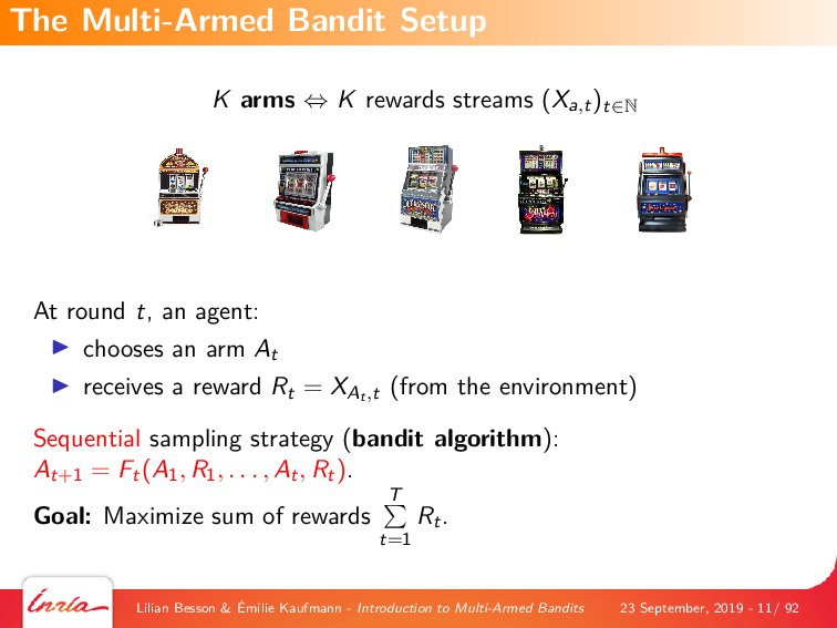
First part (Lilian BESSON): Introduction to Multi-Armed Bandits and Reinforcement Learning

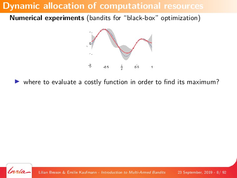
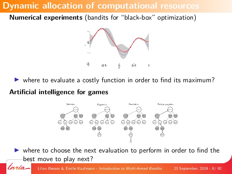
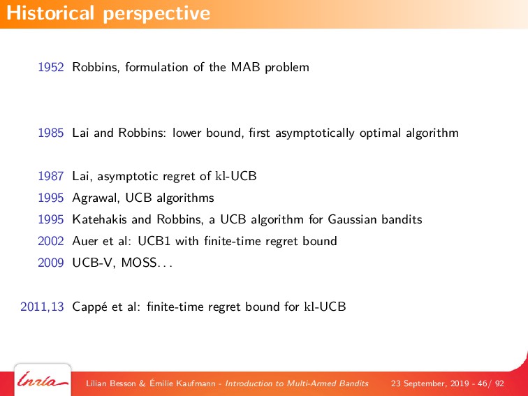
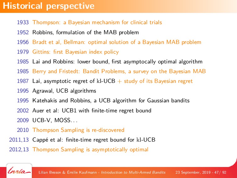
The first part of the tutorial introduces the general framework of machine learning, and focuses on reinforcement learning. We explain the model of multi-armed bandits (MAB), and we give an overview of different successful applications of MAB, since the 1950s.

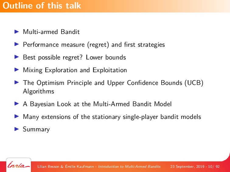
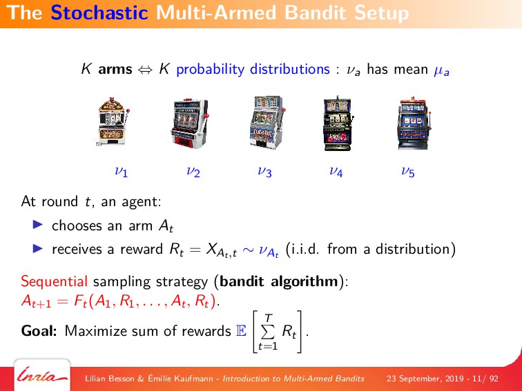
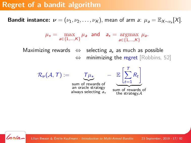
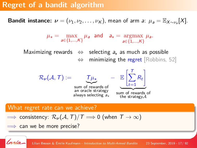
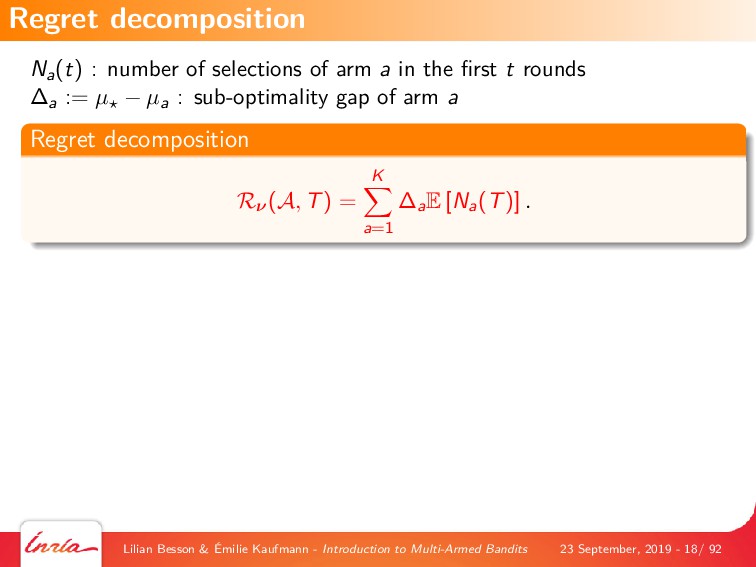
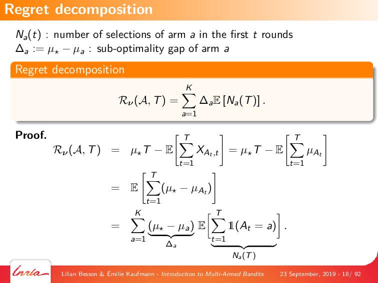
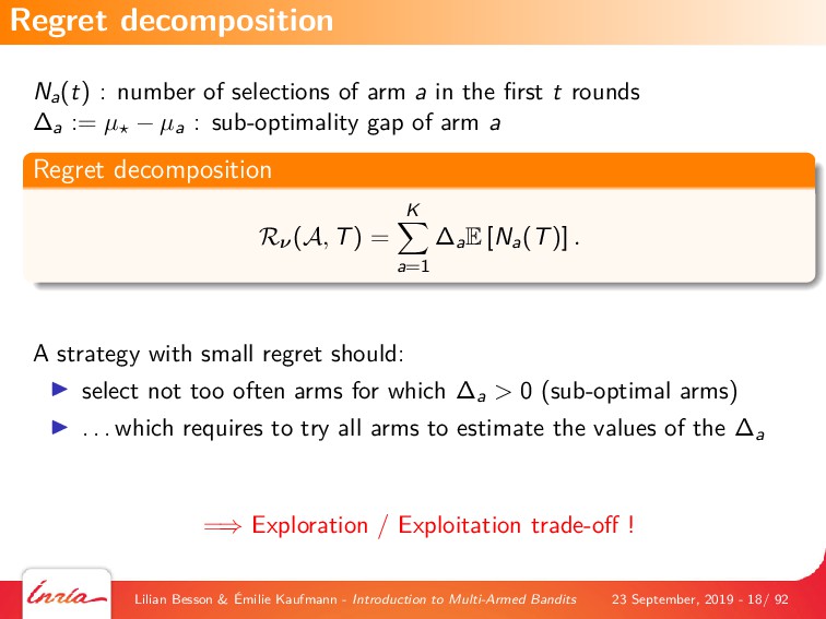
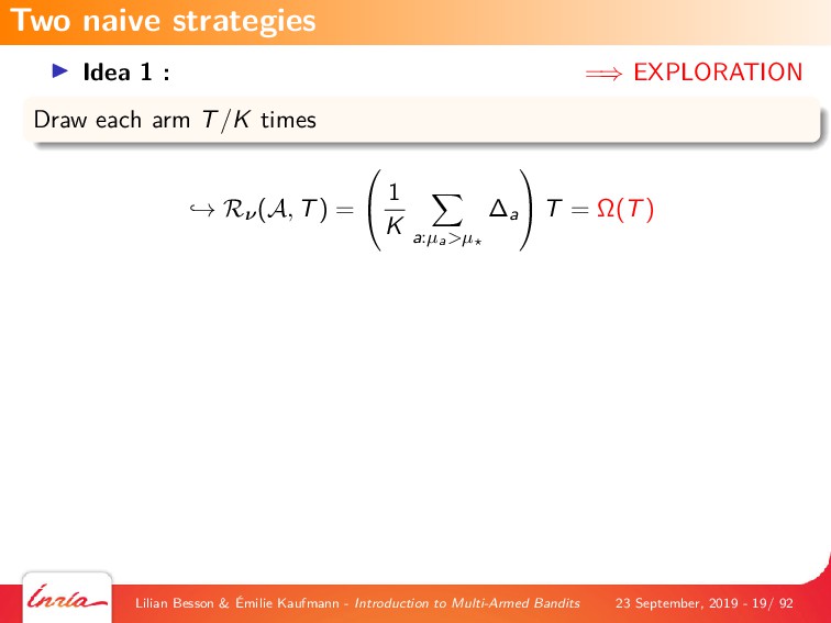
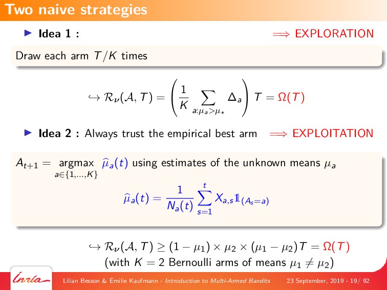
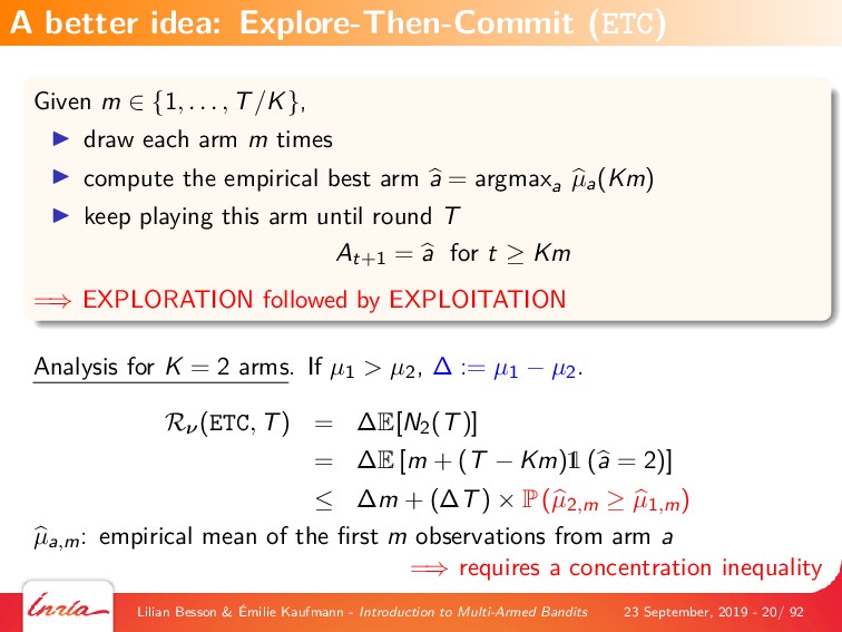
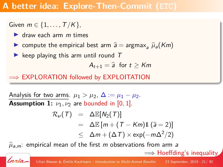
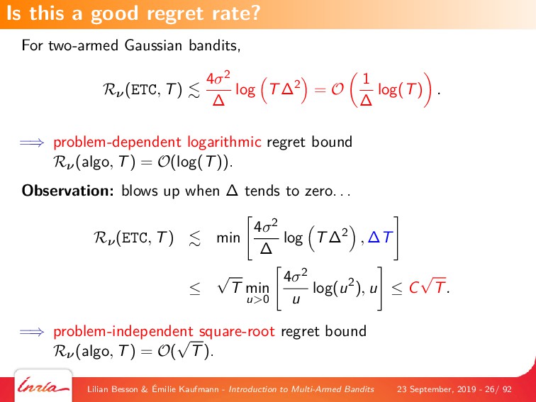
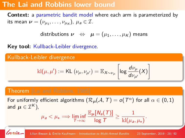
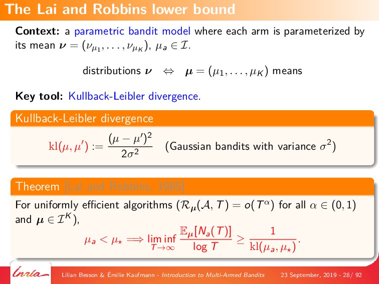
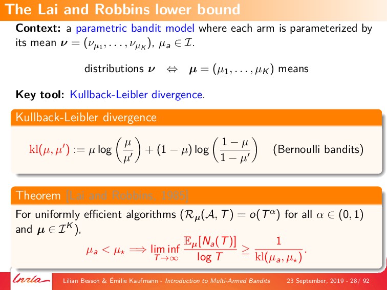
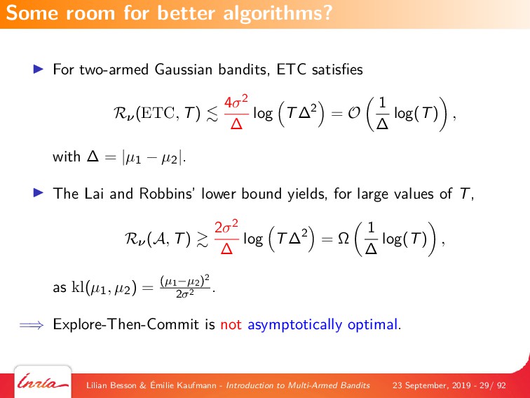
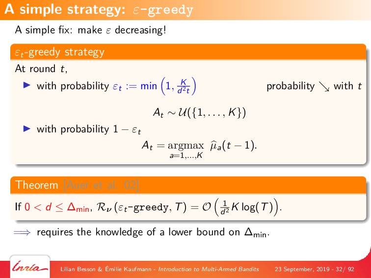
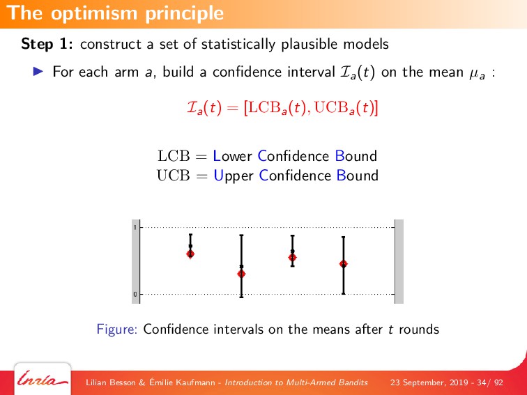
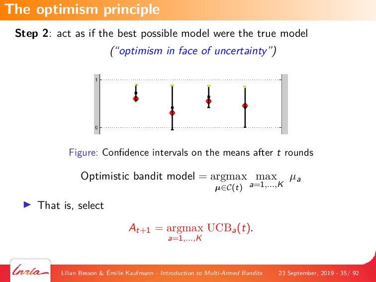
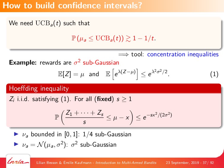
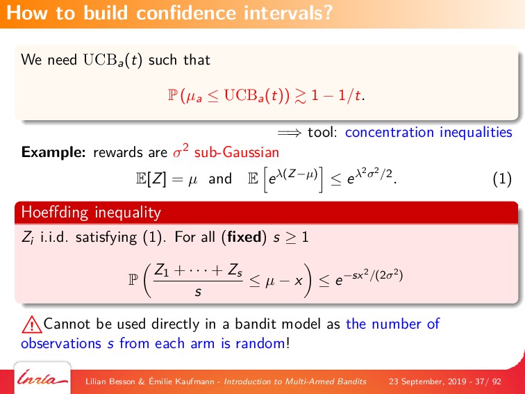
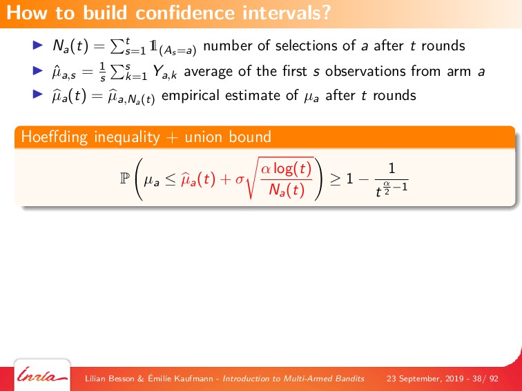
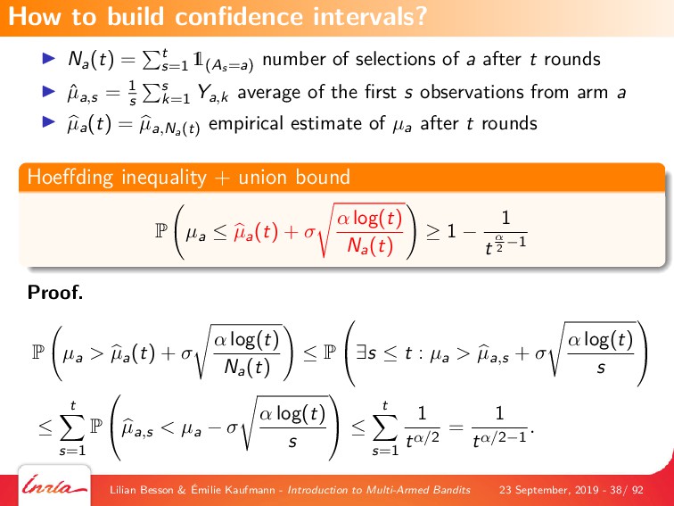
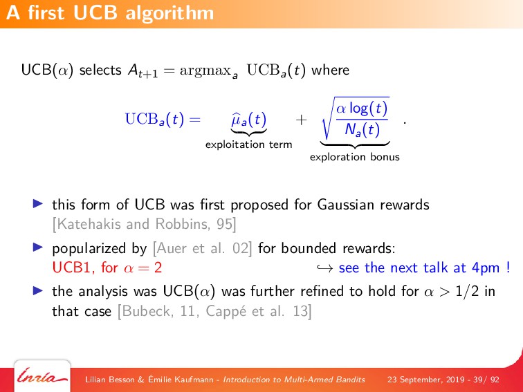
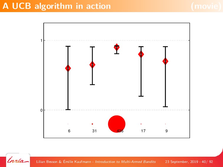
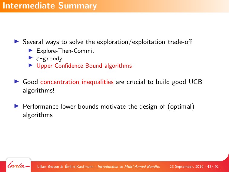
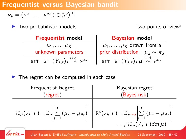
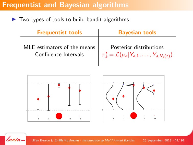
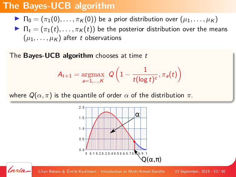
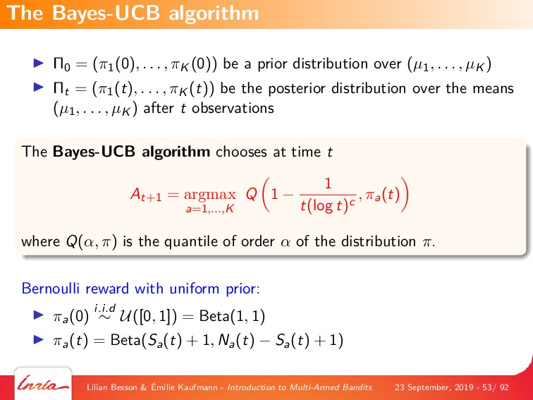
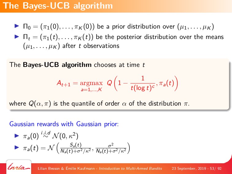
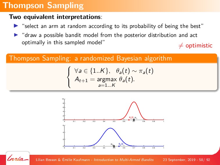
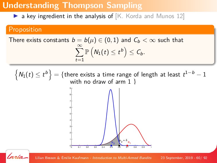
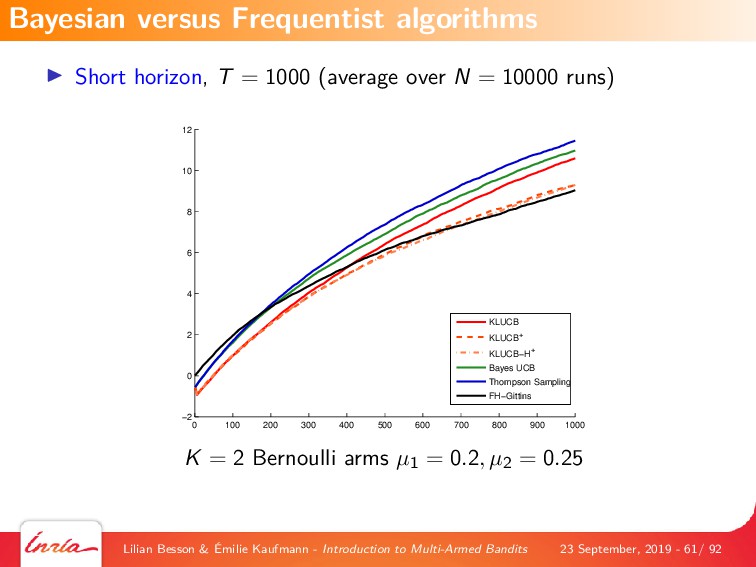
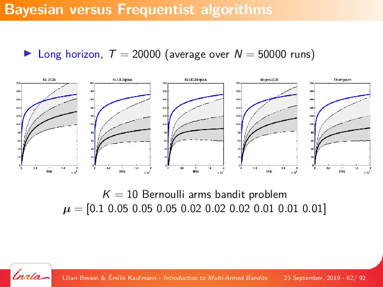
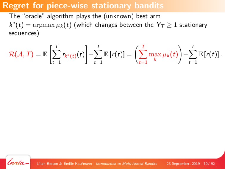
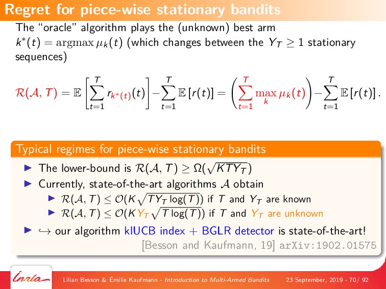
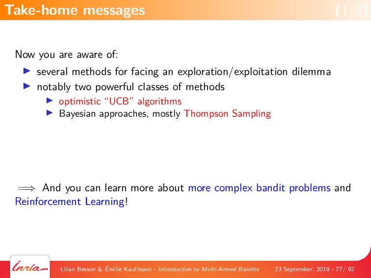
By first focusing on the simplest model, of a single player interacting with a stationary and stochastic (i.i.d) bandit game with a finite number of resources (or arms), we explain the most famous algorithms that are based on either a frequentist point-of-view, with Upper-Confidence Bounds (UCB) index policies (UCB1 and kl-UCB), or a Bayesian point-of-view, with Thompson Sampling. We also give details on the theoretical analyses of this model, by introducing the notion of regret which is a measure of performance of a MAB algorithm, and famous results from the literature on MAB algorithms, covering both what no algorithm can achieve (ie, lower-bounds on the performance on any algorithm), and what a good algorithm can indeed achieve (ie, upper-bounds on the performance of some efficient algorithms).

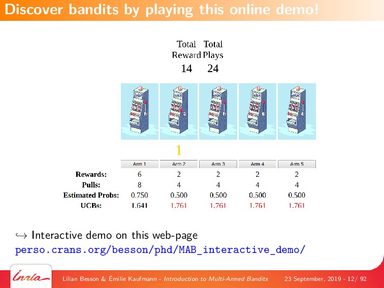
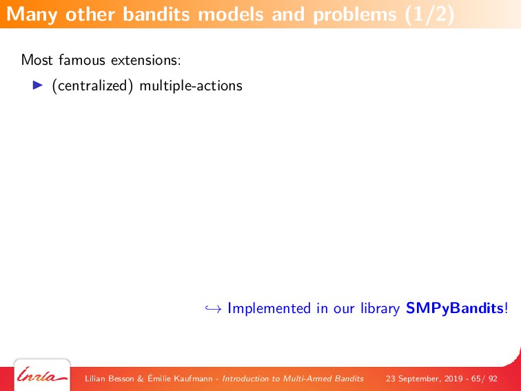
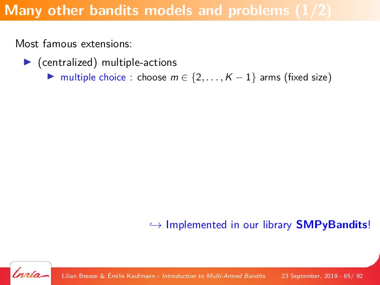
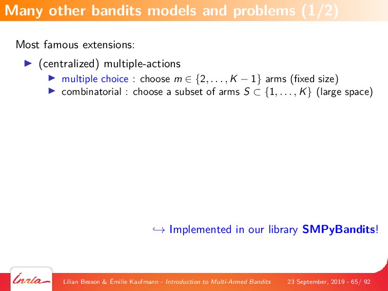
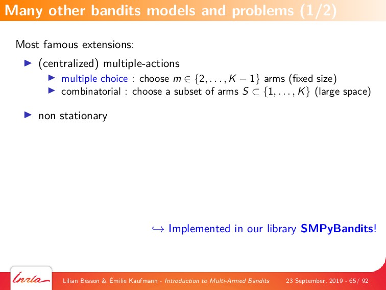
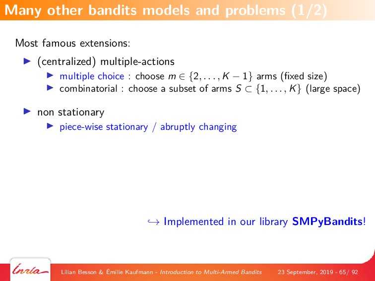
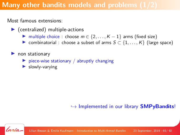
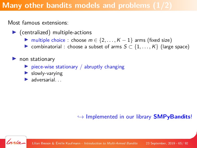
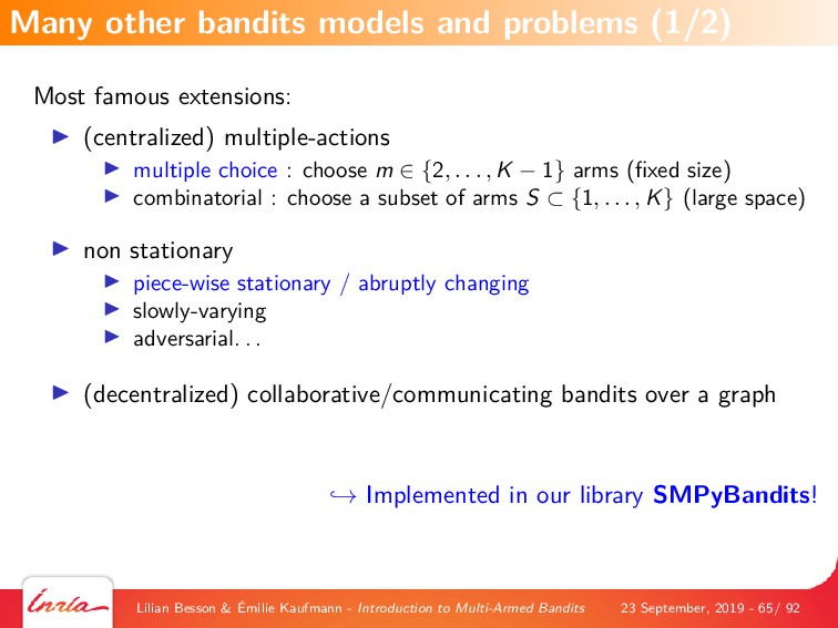
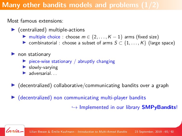
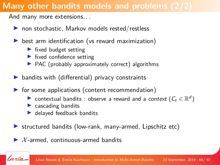
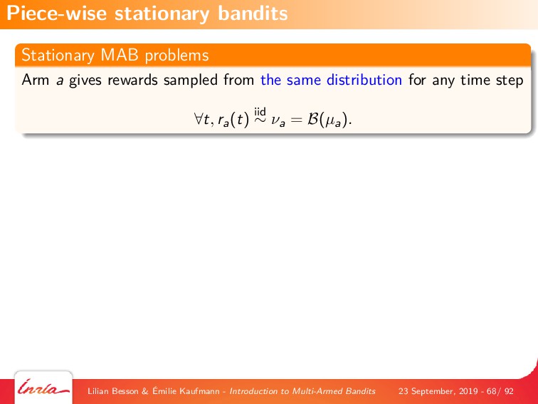
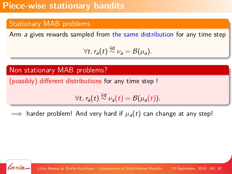
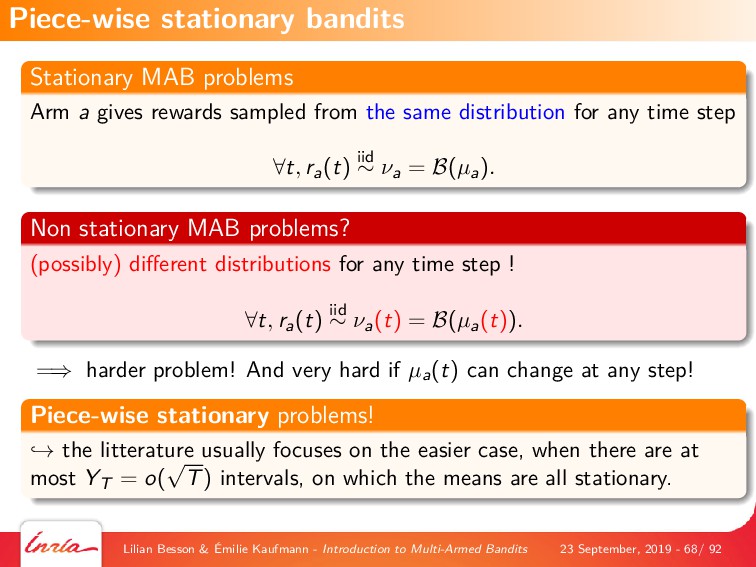
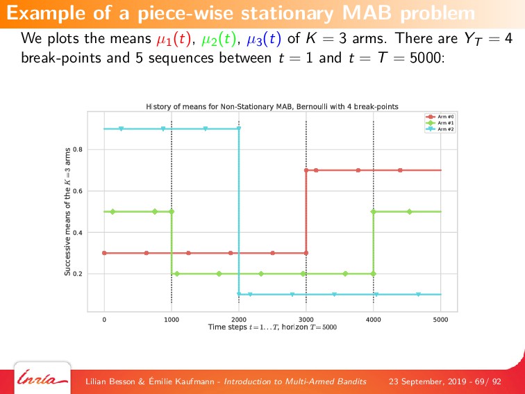
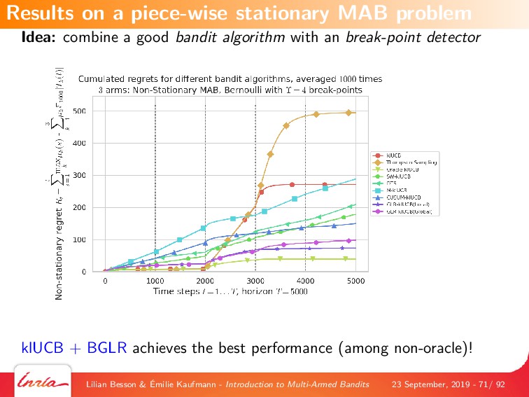
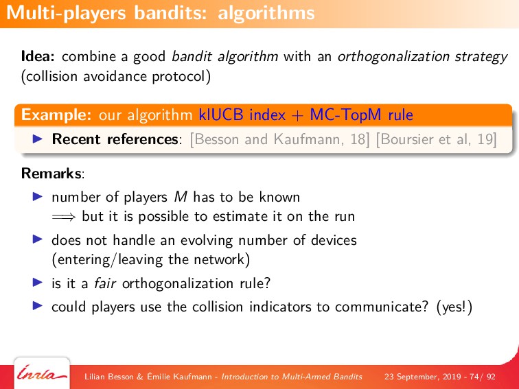
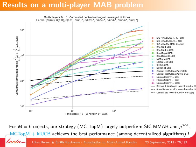
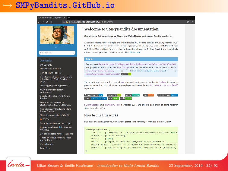
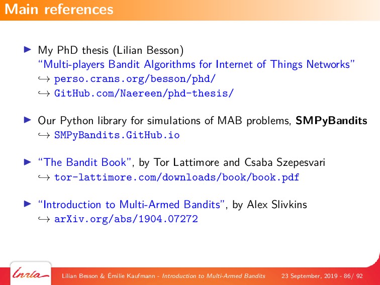
We also introduce some generalizations of this first MAB model, by considering non-stationary stochastic environments, Markov models (either rested or restless), and multi-player models. Each variant is illustrated with numerical experiments, showcasing the most well-known and most efficient algorithms, using our state-of-the-art open-source library for numerical simulations of MAB problems, SMPyBandits (see https://SMPyBandits.github.io/).

PDF : https://perso.crans.org/besson/slides/2019_09__Tutorial_on_RL_and_MAB_at_Training_School_in_Paris/slides.pdf

Transcript

1. Introduction to Multi-Armed Bandits and Reinforcement Learning Training School on Machine Learning for Communications Paris, 23-25 September 2019
2. Hi, I’m Lilian Besson finishing my PhD in telecommunication and machine learning under supervision of Prof. Christophe Moy at IETR & CentraleSupélec in Rennes (France) and Dr. Émilie Kaufmann in Inria in Lille Thanks to Émilie Kaufmann for most of the slides material! Lilian.Besson @ Inria.fr → perso.crans.org/besson/ & GitHub.com/Naereen Lilian Besson & Émilie Kaufmann - Introduction to Multi-Armed Bandits 23 September, 2019 - 2/ 92 . Who am I ?
3. It’s an old name for a casino machine! → c Dargaud, Lucky Luke tome 18. Lilian Besson & Émilie Kaufmann - Introduction to Multi-Armed Bandits 23 September, 2019 - 3/ 92 . What is a bandit?
4. Why Bandits? Lilian Besson & Émilie Kaufmann - Introduction to Multi-Armed Bandits 23 September, 2019 - 4/ 92
5. A (single) agent facing (multiple) arms in a Multi-Armed Bandit. Lilian Besson & Émilie Kaufmann - Introduction to Multi-Armed Bandits 23 September, 2019 - 5/ 92 . Make money in a casino?
6. A (single) agent facing (multiple) arms in a Multi-Armed Bandit. NO! Lilian Besson & Émilie Kaufmann - Introduction to Multi-Armed Bandits 23 September, 2019 - 5/ 92 . Make money in a casino?
7. Clinical trials K treatments for a given symptom (with unknown effect) What treatment should be allocated to the next patient, based on responses observed on previous patients? Lilian Besson & Émilie Kaufmann - Introduction to Multi-Armed Bandits 23 September, 2019 - 6/ 92 . Sequential resource allocation
8. Clinical trials K treatments for a given symptom (with unknown effect) What treatment should be allocated to the next patient, based on responses observed on previous patients? Online advertisement K adds that can be displayed Which add should be displayed for a user, based on the previous clicks of previous (similar) users? Lilian Besson & Émilie Kaufmann - Introduction to Multi-Armed Bandits 23 September, 2019 - 6/ 92 . Sequential resource allocation
9. Opportunistic Spectrum Access K radio channels (orthogonal frequency bands) In which channel should a radio device send a packet, based on the quality of its previous communications? Lilian Besson & Émilie Kaufmann - Introduction to Multi-Armed Bandits 23 September, 2019 - 7/ 92 . Dynamic channel selection
10. Opportunistic Spectrum Access K radio channels (orthogonal frequency bands) In which channel should a radio device send a packet, based on the quality of its previous communications? → see the next talk at 4pm ! Lilian Besson & Émilie Kaufmann - Introduction to Multi-Armed Bandits 23 September, 2019 - 7/ 92 . Dynamic channel selection
11. Opportunistic Spectrum Access K radio channels (orthogonal frequency bands) In which channel should a radio device send a packet, based on the quality of its previous communications? → see the next talk at 4pm ! Communications in presence of a central controller K assignments from n users to m antennas ( combinatorial bandit) How to select the next matching based on the throughput observed in previous communications? Lilian Besson & Émilie Kaufmann - Introduction to Multi-Armed Bandits 23 September, 2019 - 7/ 92 . Dynamic channel selection
12. Numerical experiments (bandits for “black-box” optimization) where to evaluate a costly function in order to find its maximum? Lilian Besson & Émilie Kaufmann - Introduction to Multi-Armed Bandits 23 September, 2019 - 8/ 92 . Dynamic allocation of computational resources
13. Numerical experiments (bandits for “black-box” optimization) where to evaluate a costly function in order to find its maximum? Artificial intelligence for games where to choose the next evaluation to perform in order to find the best move to play next? Lilian Besson & Émilie Kaufmann - Introduction to Multi-Armed Bandits 23 September, 2019 - 8/ 92 . Dynamic allocation of computational resources
14. rewards maximization in a stochastic bandit model = the simplest Reinforcement Learning (RL) problem (one state) =⇒ good introduction to RL ! bandits showcase the important exploration/exploitation dilemma bandit tools are useful for RL (UCRL, bandit-based MCTS for planning in games. . . ) a rich literature to tackle many specific applications bandits have application beyond RL (i.e. without “reward”) and bandits have great applications to Cognitive Radio → see the next talk at 4pm ! Lilian Besson & Émilie Kaufmann - Introduction to Multi-Armed Bandits 23 September, 2019 - 9/ 92 . Why talking about bandits today?
15. Multi-armed Bandit Performance measure (regret) and first strategies Best possible regret? Lower bounds Mixing Exploration and Exploitation The Optimism Principle and Upper Confidence Bounds (UCB) Algorithms A Bayesian Look at the Multi-Armed Bandit Model Many extensions of the stationary single-player bandit models Summary Lilian Besson & Émilie Kaufmann - Introduction to Multi-Armed Bandits 23 September, 2019 - 10/ 92 . Outline of this talk
16. K arms ⇔ K rewards streams (Xa,t)t∈N At round t, an agent: chooses an arm At receives a reward Rt = XAt ,t (from the environment) Sequential sampling strategy (bandit algorithm): At+1 = Ft(A1, R1, . . . , At, Rt). Goal: Maximize sum of rewards T t=1 Rt. Lilian Besson & Émilie Kaufmann - Introduction to Multi-Armed Bandits 23 September, 2019 - 11/ 92 . The Multi-Armed Bandit Setup
17. K arms ⇔ K probability distributions : νa has mean µa ν1 ν2 ν3 ν4 ν5 At round t, an agent: chooses an arm At receives a reward Rt = XAt ,t ∼ νAt (i.i.d. from a distribution) Sequential sampling strategy (bandit algorithm): At+1 = Ft(A1, R1, . . . , At, Rt). Goal: Maximize sum of rewards E T t=1 Rt . Lilian Besson & Émilie Kaufmann - Introduction to Multi-Armed Bandits 23 September, 2019 - 11/ 92 . The Stochastic Multi-Armed Bandit Setup
18. → Interactive demo on this web-page perso.crans.org/besson/phd/MAB_interactive_demo/ Lilian Besson & Émilie Kaufmann - Introduction to Multi-Armed Bandits 23 September, 2019 - 12/ 92 . Discover bandits by playing this online demo!
19. Historical motivation [Thompson 1933] B(µ1) B(µ2) B(µ3) B(µ4) B(µ5) For the t-th patient in a clinical study, chooses a treatment At observes a (Bernoulli) response Rt ∈ {0, 1} : P(Rt = 1|At = a) = µa Goal: maximize the expected number of patients healed. Lilian Besson & Émilie Kaufmann - Introduction to Multi-Armed Bandits 23 September, 2019 - 13/ 92 . Clinical trials
20. Modern motivation ($$$$) [Li et al, 2010] (recommender systems, online advertisement, etc) ν1 ν2 ν3 ν4 ν5 For the t-th visitor of a website, recommend a movie At observe a rating Rt ∼ νAt (e.g. Rt ∈ {1, . . . , 5}) Goal: maximize the sum of ratings. Lilian Besson & Émilie Kaufmann - Introduction to Multi-Armed Bandits 23 September, 2019 - 14/ 92 . Online content optimization
21. Opportunistic spectrum access [Zhao et al. 10] [Anandkumar et al. 11] streams indicating channel quality Channel 1 X1,1 X1,2 . . . X1,t . . . X1,T ∼ ν1 Channel 2 X2,1 X2,2 . . . X2,t . . . X2,T ∼ ν2 . . . . . . . . . . . . . . . . . . . . . . . . Channel K XK,1 XK,2 . . . XK,t . . . XK,T ∼ νK At round t, the device: selects a channel At observes the quality of its communication Rt = XAt ,t ∈ [0, 1] Goal: Maximize the overall quality of communications. → see the next talk at 4pm ! Lilian Besson & Émilie Kaufmann - Introduction to Multi-Armed Bandits 23 September, 2019 - 15/ 92 . Cognitive radios
22. Performance measure and first strategies Lilian Besson & Émilie Kaufmann - Introduction to Multi-Armed Bandits 23 September, 2019 - 16/ 92
23. Bandit instance: ν = (ν1, ν2, . . . , νK ), mean of arm a: µa = EX∼νa [X]. µ = max a∈{1,...,K} µa and a = argmax a∈{1,...,K} µa. Maximizing rewards ⇔ selecting a as much as possible ⇔ minimizing the regret [Robbins, 52] Rν(A, T) := Tµ sum of rewards of an oracle strategy always selecting a − E T t=1 Rt sum of rewards of the strategyA Lilian Besson & Émilie Kaufmann - Introduction to Multi-Armed Bandits 23 September, 2019 - 17/ 92 . Regret of a bandit algorithm
24. Bandit instance: ν = (ν1, ν2, . . . , νK ), mean of arm a: µa = EX∼νa [X]. µ = max a∈{1,...,K} µa and a = argmax a∈{1,...,K} µa. Maximizing rewards ⇔ selecting a as much as possible ⇔ minimizing the regret [Robbins, 52] Rν(A, T) := Tµ sum of rewards of an oracle strategy always selecting a − E T t=1 Rt sum of rewards of the strategyA What regret rate can we achieve? =⇒ consistency: Rν(A, T)/T =⇒ 0 (when T → ∞) =⇒ can we be more precise? Lilian Besson & Émilie Kaufmann - Introduction to Multi-Armed Bandits 23 September, 2019 - 17/ 92 . Regret of a bandit algorithm
25. Na(t) : number of selections of arm a in the first t rounds ∆a := µ − µa : sub-optimality gap of arm a Regret decomposition Rν(A, T) = K a=1 ∆aE [Na(T)] . Lilian Besson & Émilie Kaufmann - Introduction to Multi-Armed Bandits 23 September, 2019 - 18/ 92 . Regret decomposition
26. Na(t) : number of selections of arm a in the first t rounds ∆a := µ − µa : sub-optimality gap of arm a Regret decomposition Rν(A, T) = K a=1 ∆aE [Na(T)] . Proof. Rν(A, T) = µ T − E T t=1 XAt ,t = µ T − E T t=1 µAt = E T t=1 (µ − µAt ) = K a=1 (µ − µa) ∆a E T t=1 1(At = a) Na(T) . Lilian Besson & Émilie Kaufmann - Introduction to Multi-Armed Bandits 23 September, 2019 - 18/ 92 . Regret decomposition
27. Na(t) : number of selections of arm a in the first t rounds ∆a := µ − µa : sub-optimality gap of arm a Regret decomposition Rν(A, T) = K a=1 ∆aE [Na(T)] . A strategy with small regret should: select not too often arms for which ∆a > 0 (sub-optimal arms) . . . which requires to try all arms to estimate the values of the ∆a =⇒ Exploration / Exploitation trade-off ! Lilian Besson & Émilie Kaufmann - Introduction to Multi-Armed Bandits 23 September, 2019 - 18/ 92 . Regret decomposition
28. Idea 1 : =⇒ EXPLORATION Draw each arm T/K times → Rν(A, T) =   1 K a:µa>µ ∆a   T = Ω(T) Lilian Besson & Émilie Kaufmann - Introduction to Multi-Armed Bandits 23 September, 2019 - 19/ 92 . Two naive strategies
29. Idea 1 : =⇒ EXPLORATION Draw each arm T/K times → Rν(A, T) =   1 K a:µa>µ ∆a   T = Ω(T) Idea 2 : Always trust the empirical best arm =⇒ EXPLOITATION At+1 = argmax a∈{1,...,K} µa(t) using estimates of the unknown means µa µa(t) = 1 Na(t) t s=1 Xa,s1(As =a) → Rν(A, T) ≥ (1 − µ1) × µ2 × (µ1 − µ2)T = Ω(T) (with K = 2 Bernoulli arms of means µ1 = µ2) Lilian Besson & Émilie Kaufmann - Introduction to Multi-Armed Bandits 23 September, 2019 - 19/ 92 . Two naive strategies
30. Given m ∈ {1, . . . , T/K}, draw each arm m times compute the empirical best arm a = argmaxa µa(Km) keep playing this arm until round T At+1 = a for t ≥ Km =⇒ EXPLORATION followed by EXPLOITATION Lilian Besson & Émilie Kaufmann - Introduction to Multi-Armed Bandits 23 September, 2019 - 20/ 92 . A better idea: Explore-Then-Commit (ETC)
31. Given m ∈ {1, . . . , T/K}, draw each arm m times compute the empirical best arm a = argmaxa µa(Km) keep playing this arm until round T At+1 = a for t ≥ Km =⇒ EXPLORATION followed by EXPLOITATION Analysis for K = 2 arms. If µ1 > µ2, ∆ := µ1 − µ2. Rν(ETC, T) = ∆E[N2(T)] = ∆E [m + (T − Km)1 (a = 2)] ≤ ∆m + (∆T) × P (µ2,m ≥ µ1,m) µa,m: empirical mean of the first m observations from arm a Lilian Besson & Émilie Kaufmann - Introduction to Multi-Armed Bandits 23 September, 2019 - 20/ 92 . A better idea: Explore-Then-Commit (ETC)
32. Given m ∈ {1, . . . , T/K}, draw each arm m times compute the empirical best arm a = argmaxa µa(Km) keep playing this arm until round T At+1 = a for t ≥ Km =⇒ EXPLORATION followed by EXPLOITATION Analysis for K = 2 arms. If µ1 > µ2, ∆ := µ1 − µ2. Rν(ETC, T) = ∆E[N2(T)] = ∆E [m + (T − Km)1 (a = 2)] ≤ ∆m + (∆T) × P (µ2,m ≥ µ1,m) µa,m: empirical mean of the first m observations from arm a =⇒ requires a concentration inequality Lilian Besson & Émilie Kaufmann - Introduction to Multi-Armed Bandits 23 September, 2019 - 20/ 92 . A better idea: Explore-Then-Commit (ETC)
33. Given m ∈ {1, . . . , T/K}, draw each arm m times compute the empirical best arm a = argmaxa µa(Km) keep playing this arm until round T At+1 = a for t ≥ Km =⇒ EXPLORATION followed by EXPLOITATION Analysis for two arms. µ1 > µ2, ∆ := µ1 − µ2. Assumption 1: ν1, ν2 are bounded in [0, 1]. Rν(T) = ∆E[N2(T)] = ∆E [m + (T − Km)1 (a = 2)] ≤ ∆m + (∆T) × exp(−m∆2/2) µa,m: empirical mean of the first m observations from arm a =⇒ Hoeffding’s inequality Lilian Besson & Émilie Kaufmann - Introduction to Multi-Armed Bandits 23 September, 2019 - 21/ 92 . A better idea: Explore-Then-Commit (ETC)
34. Given m ∈ {1, . . . , T/K}, draw each arm m times compute the empirical best arm a = argmaxa µa(Km) keep playing this arm until round T At+1 = a for t ≥ Km =⇒ EXPLORATION followed by EXPLOITATION Analysis for two arms. µ1 > µ2, ∆ := µ1 − µ2. Assumption 2: ν1 = N(µ1, σ2), ν2 = N(µ2, σ2) are Gaussian arms. Rν(ETC, T) = ∆E[N2(T)] = ∆E [m + (T − Km)1 (a = 2)] ≤ ∆m + (∆T) × exp(−m∆2/4σ2) µa,m: empirical mean of the first m observations from arm a =⇒ Gaussian tail inequality Lilian Besson & Émilie Kaufmann - Introduction to Multi-Armed Bandits 23 September, 2019 - 22/ 92 . A better idea: Explore-Then-Commit (ETC)
35. Given m ∈ {1, . . . , T/K}, draw each arm m times compute the empirical best arm a = argmaxa µa(Km) keep playing this arm until round T At+1 = a for t ≥ Km =⇒ EXPLORATION followed by EXPLOITATION Analysis for two arms. µ1 > µ2, ∆ := µ1 − µ2. Assumption 2: ν1 = N(µ1, σ2), ν2 = N(µ2, σ2) are Gaussian arms. Rν(ETC, T) = ∆E[N2(T)] = ∆E [m + (T − Km)1 (a = 2)] ≤ ∆m + (∆T) × exp(−m∆2/4σ2) µa,m: empirical mean of the first m observations from arm a =⇒ Gaussian tail inequality Lilian Besson & Émilie Kaufmann - Introduction to Multi-Armed Bandits 23 September, 2019 - 22/ 92 . A better idea: Explore-Then-Commit (ETC)
36. Given m ∈ {1, . . . , T/K}, draw each arm m times compute the empirical best arm a = argmaxa µa(Km) keep playing this arm until round T At+1 = a for t ≥ Km =⇒ EXPLORATION followed by EXPLOITATION Analysis for two arms. µ1 > µ2, ∆ := µ1 − µ2. Assumption: ν1 = N(µ1, σ2), ν2 = N(µ2, σ2) are Gaussian arms. For m = 4σ2 ∆2 log T∆2 4σ2 , Rν(ETC, T) ≤ 4σ2 ∆ log T∆2 2 + 1 = O 1 ∆ log(T) . Lilian Besson & Émilie Kaufmann - Introduction to Multi-Armed Bandits 23 September, 2019 - 23/ 92 . A better idea: Explore-Then-Commit (ETC)
37. Given m ∈ {1, . . . , T/K}, draw each arm m times compute the empirical best arm a = argmaxa µa(Km) keep playing this arm until round T At+1 = a for t ≥ Km =⇒ EXPLORATION followed by EXPLOITATION Analysis for two arms. µ1 > µ2, ∆ := µ1 − µ2. Assumption: ν1 = N(µ1, σ2), ν2 = N(µ2, σ2) are Gaussian arms. For m = 4σ2 ∆2 log T∆2 4σ2 , Rν(ETC, T) ≤ 4σ2 ∆ log T∆2 2 + 1 = O 1 ∆ log(T) . + logarithmic regret! − requires the knowledge of T ( OKAY) and ∆ (NOT OKAY) Lilian Besson & Émilie Kaufmann - Introduction to Multi-Armed Bandits 23 September, 2019 - 23/ 92 . A better idea: Explore-Then-Commit (ETC)
38. explore uniformly until the random time τ = inf    t ∈ N : |µ1(t) − µ2(t)| > 8σ2 log(T/t) t    0 200 400 600 800 1000 −1.0 −0.5 0.0 0.5 1.0 aτ = argmax a µa(τ) and (At+1 = aτ ) for t ∈ {τ + 1, . . . , T} Rν(S-ETC, T) ≤ 4σ2 ∆ log T∆2 + C log(T) = O 1 ∆ log(T) . =⇒ same regret rate, without knowing ∆ [Garivier et al. 2016] Lilian Besson & Émilie Kaufmann - Introduction to Multi-Armed Bandits 23 September, 2019 - 24/ 92 . Sequential Explore-Then-Commit (2 Gaussian arms)
39. Two Gaussian arms: ν1 = N(1, 1) and ν2 = N(1.5, 1) 0 200 400 600 800 1000 0 100 200 300 400 500 Uniform FTL Sequential-ETC 0 200 400 600 800 1000 0 5 10 15 20 25 30 35 40 Sequential-ETC Expected regret estimated over N = 500 runs for Sequential-ETC versus our two naive baselines. (dashed lines: empirical 0.05% and 0.95% quantiles of the regret) Lilian Besson & Émilie Kaufmann - Introduction to Multi-Armed Bandits 23 September, 2019 - 25/ 92 . Numerical illustration
40. For two-armed Gaussian bandits, Rν(ETC, T) 4σ2 ∆ log T∆2 = O 1 ∆ log(T) . =⇒ problem-dependent logarithmic regret bound Rν(algo, T) = O(log(T)). Observation: blows up when ∆ tends to zero. . . Rν(ETC, T) min 4σ2 ∆ log T∆2 , ∆T ≤ √ T min u>0 4σ2 u log(u2), u ≤ C √ T. =⇒ problem-independent square-root regret bound Rν(algo, T) = O( √ T). Lilian Besson & Émilie Kaufmann - Introduction to Multi-Armed Bandits 23 September, 2019 - 26/ 92 . Is this a good regret rate?
41. Best possible regret? Lower Bounds Lilian Besson & Émilie Kaufmann - Introduction to Multi-Armed Bandits 23 September, 2019 - 27/ 92
42. Context: a parametric bandit model where each arm is parameterized by its mean ν = (νµ1 , . . . , νµK ), µa ∈ I. distributions ν ⇔ µ = (µ1, . . . , µK ) means Key tool: Kullback-Leibler divergence. Kullback-Leibler divergence kl(µ, µ ) := KL νµ, νµ = EX∼νµ log dνµ dνµ (X) Theorem [Lai and Robbins, 1985] For uniformly efficient algorithms (Rµ(A, T) = o(Tα) for all α ∈ (0, 1) and µ ∈ IK ), µa < µ =⇒ lim inf T→∞ Eµ[Na(T)] log T ≥ 1 kl(µa, µ ) . Lilian Besson & Émilie Kaufmann - Introduction to Multi-Armed Bandits 23 September, 2019 - 28/ 92 . The Lai and Robbins lower bound
43. Context: a parametric bandit model where each arm is parameterized by its mean ν = (νµ1 , . . . , νµK ), µa ∈ I. distributions ν ⇔ µ = (µ1, . . . , µK ) means Key tool: Kullback-Leibler divergence. Kullback-Leibler divergence kl(µ, µ ) := (µ − µ )2 2σ2 (Gaussian bandits with variance σ2) Theorem [Lai and Robbins, 1985] For uniformly efficient algorithms (Rµ(A, T) = o(Tα) for all α ∈ (0, 1) and µ ∈ IK ), µa < µ =⇒ lim inf T→∞ Eµ[Na(T)] log T ≥ 1 kl(µa, µ ) . Lilian Besson & Émilie Kaufmann - Introduction to Multi-Armed Bandits 23 September, 2019 - 28/ 92 . The Lai and Robbins lower bound
44. Context: a parametric bandit model where each arm is parameterized by its mean ν = (νµ1 , . . . , νµK ), µa ∈ I. distributions ν ⇔ µ = (µ1, . . . , µK ) means Key tool: Kullback-Leibler divergence. Kullback-Leibler divergence kl(µ, µ ) := µ log µ µ + (1 − µ) log 1 − µ 1 − µ (Bernoulli bandits) Theorem [Lai and Robbins, 1985] For uniformly efficient algorithms (Rµ(A, T) = o(Tα) for all α ∈ (0, 1) and µ ∈ IK ), µa < µ =⇒ lim inf T→∞ Eµ[Na(T)] log T ≥ 1 kl(µa, µ ) . Lilian Besson & Émilie Kaufmann - Introduction to Multi-Armed Bandits 23 September, 2019 - 28/ 92 . The Lai and Robbins lower bound
45. For two-armed Gaussian bandits, ETC satisfies Rν(ETC, T) 4σ2 ∆ log T∆2 = O 1 ∆ log(T) , with ∆ = |µ1 − µ2|. The Lai and Robbins’ lower bound yields, for large values of T, Rν(A, T) 2σ2 ∆ log T∆2 = Ω 1 ∆ log(T) , as kl(µ1, µ2) = (µ1−µ2)2 2σ2 . =⇒ Explore-Then-Commit is not asymptotically optimal. Lilian Besson & Émilie Kaufmann - Introduction to Multi-Armed Bandits 23 September, 2019 - 29/ 92 . Some room for better algorithms?
46. Mixing Exploration and Exploitation Lilian Besson & Émilie Kaufmann - Introduction to Multi-Armed Bandits 23 September, 2019 - 30/ 92
47. The ε-greedy rule [Sutton and Barton, 98] is the simplest way to alternate exploration and exploitation. ε-greedy strategy At round t, with probability ε At ∼ U({1, . . . , K}) with probability 1 − ε At = argmax a=1,...,K µa(t). =⇒ Linear regret: Rν (ε-greedy, T) ≥ εK−1 K ∆minT. ∆min = min a:µa<µ ∆a. Lilian Besson & Émilie Kaufmann - Introduction to Multi-Armed Bandits 23 September, 2019 - 31/ 92 . A simple strategy: ε-greedy
48. A simple fix: make ε decreasing! εt -greedy strategy At round t, with probability εt := min 1, K d2t probability with t At ∼ U({1, . . . , K}) with probability 1 − εt At = argmax a=1,...,K µa(t − 1). Theorem [Auer et al. 02] If 0 < d ≤ ∆min, Rν (εt-greedy, T) = O 1 d2 K log(T) . =⇒ requires the knowledge of a lower bound on ∆min. Lilian Besson & Émilie Kaufmann - Introduction to Multi-Armed Bandits 23 September, 2019 - 32/ 92 . A simple strategy: ε-greedy
49. The Optimism Principle Upper Confidence Bounds Algorithms Lilian Besson & Émilie Kaufmann - Introduction to Multi-Armed Bandits 23 September, 2019 - 33/ 92
50. Step 1: construct a set of statistically plausible models For each arm a, build a confidence interval Ia(t) on the mean µa : Ia(t) = [LCBa(t), UCBa(t)] LCB = Lower Confidence Bound UCB = Upper Confidence Bound Figure: Confidence intervals on the means after t rounds Lilian Besson & Émilie Kaufmann - Introduction to Multi-Armed Bandits 23 September, 2019 - 34/ 92 . The optimism principle
51. Step 2: act as if the best possible model were the true model (“optimism in face of uncertainty”) Figure: Confidence intervals on the means after t rounds Optimistic bandit model = argmax µ∈C(t) max a=1,...,K µa That is, select At+1 = argmax a=1,...,K UCBa(t). Lilian Besson & Émilie Kaufmann - Introduction to Multi-Armed Bandits 23 September, 2019 - 35/ 92 . The optimism principle
52. Optimistic Algorithms Building Confidence Intervals Analysis of UCB(α) Lilian Besson & Émilie Kaufmann - Introduction to Multi-Armed Bandits 23 September, 2019 - 36/ 92
53. We need UCBa(t) such that P (µa ≤ UCBa(t)) 1 − 1/t. =⇒ tool: concentration inequalities Example: rewards are σ2 sub-Gaussian E[Z] = µ and E eλ(Z−µ) ≤ eλ2σ2/2. (1) Hoeffding inequality Zi i.i.d. satisfying (1). For all (fixed) s ≥ 1 P Z1 + · · · + Zs s ≥ µ + x ≤ e−sx2/(2σ2) νa bounded in [0, 1]: 1/4 sub-Gaussian νa = N(µa, σ2): σ2 sub-Gaussian Lilian Besson & Émilie Kaufmann - Introduction to Multi-Armed Bandits 23 September, 2019 - 37/ 92 . How to build confidence intervals?
54. We need UCBa(t) such that P (µa ≤ UCBa(t)) 1 − 1/t. =⇒ tool: concentration inequalities Example: rewards are σ2 sub-Gaussian E[Z] = µ and E eλ(Z−µ) ≤ eλ2σ2/2. (1) Hoeffding inequality Zi i.i.d. satisfying (1). For all (fixed) s ≥ 1 P Z1 + · · · + Zs s ≤ µ − x ≤ e−sx2/(2σ2) νa bounded in [0, 1]: 1/4 sub-Gaussian νa = N(µa, σ2): σ2 sub-Gaussian Lilian Besson & Émilie Kaufmann - Introduction to Multi-Armed Bandits 23 September, 2019 - 37/ 92 . How to build confidence intervals?
55. We need UCBa(t) such that P (µa ≤ UCBa(t)) 1 − 1/t. =⇒ tool: concentration inequalities Example: rewards are σ2 sub-Gaussian E[Z] = µ and E eλ(Z−µ) ≤ eλ2σ2/2. (1) Hoeffding inequality Zi i.i.d. satisfying (1). For all (fixed) s ≥ 1 P Z1 + · · · + Zs s ≤ µ − x ≤ e−sx2/(2σ2) Cannot be used directly in a bandit model as the number of observations s from each arm is random! Lilian Besson & Émilie Kaufmann - Introduction to Multi-Armed Bandits 23 September, 2019 - 37/ 92 . How to build confidence intervals?
56. Na(t) = t s=1 1(As =a) number of selections of a after t rounds ˆ µa,s = 1 s s k=1 Ya,k average of the first s observations from arm a µa(t) = µa,Na(t) empirical estimate of µa after t rounds Hoeffding inequality + union bound P µa ≤ µa(t) + σ α log(t) Na(t) ≥ 1 − 1 t α 2 −1 Lilian Besson & Émilie Kaufmann - Introduction to Multi-Armed Bandits 23 September, 2019 - 38/ 92 . How to build confidence intervals?
57. Na(t) = t s=1 1(As =a) number of selections of a after t rounds ˆ µa,s = 1 s s k=1 Ya,k average of the first s observations from arm a µa(t) = µa,Na(t) empirical estimate of µa after t rounds Hoeffding inequality + union bound P µa ≤ µa(t) + σ α log(t) Na(t) ≥ 1 − 1 t α 2 −1 Proof. P µa > µa(t) + σ α log(t) Na(t) ≤ P  ∃s ≤ t : µa > µa,s + σ α log(t) s   ≤ t s=1 P  µa,s < µa − σ α log(t) s   ≤ t s=1 1 tα/2 = 1 tα/2−1 . Lilian Besson & Émilie Kaufmann - Introduction to Multi-Armed Bandits 23 September, 2019 - 38/ 92 . How to build confidence intervals?
58. UCB(α) selects At+1 = argmaxa UCBa(t) where UCBa(t) = µa(t) exploitation term + α log(t) Na(t) exploration bonus . this form of UCB was first proposed for Gaussian rewards [Katehakis and Robbins, 95] popularized by [Auer et al. 02] for bounded rewards: UCB1, for α = 2 → see the next talk at 4pm ! the analysis was UCB(α) was further refined to hold for α > 1/2 in that case [Bubeck, 11, Cappé et al. 13] Lilian Besson & Émilie Kaufmann - Introduction to Multi-Armed Bandits 23 September, 2019 - 39/ 92 . A first UCB algorithm
59. 0 1 6 31 436 17 9 Lilian Besson & Émilie Kaufmann - Introduction to Multi-Armed Bandits 23 September, 2019 - 40/ 92 . A UCB algorithm in action (movie)
60. Optimistic Algorithms Building Confidence Intervals Analysis of UCB(α) Lilian Besson & Émilie Kaufmann - Introduction to Multi-Armed Bandits 23 September, 2019 - 41/ 92
61. Theorem [Auer et al, 02] UCB(α) with parameter α = 2 satisfies Rν(UCB1, T) ≤ 8   a:µa<µ 1 ∆a   log(T) + 1 + π2 3 K a=1 ∆a . Theorem For every α > 1 and every sub-optimal arm a, there exists a constant Cα > 0 such that Eµ[Na(T)] ≤ 4α (µ − µa)2 log(T) + Cα. It follows that Rν(UCB(α), T) ≤ 4α   a:µa<µ 1 ∆a   log(T) + KCα. Lilian Besson & Émilie Kaufmann - Introduction to Multi-Armed Bandits 23 September, 2019 - 42/ 92 . Regret of UCB(α) for bounded rewards
62. Several ways to solve the exploration/exploitation trade-off Explore-Then-Commit ε-greedy Upper Confidence Bound algorithms Good concentration inequalities are crucial to build good UCB algorithms! Performance lower bounds motivate the design of (optimal) algorithms Lilian Besson & Émilie Kaufmann - Introduction to Multi-Armed Bandits 23 September, 2019 - 43/ 92 . Intermediate Summary
63. A Bayesian Look at the MAB Model Lilian Besson & Émilie Kaufmann - Introduction to Multi-Armed Bandits 23 September, 2019 - 44/ 92
64. Bayesian Bandits Two points of view Bayes-UCB Thompson Sampling Lilian Besson & Émilie Kaufmann - Introduction to Multi-Armed Bandits 23 September, 2019 - 45/ 92
65. 1952 Robbins, formulation of the MAB problem 1985 Lai and Robbins: lower bound, first asymptotically optimal algorithm 1987 Lai, asymptotic regret of kl-UCB 1995 Agrawal, UCB algorithms 1995 Katehakis and Robbins, a UCB algorithm for Gaussian bandits 2002 Auer et al: UCB1 with finite-time regret bound 2009 UCB-V, MOSS. . . 2011,13 Cappé et al: finite-time regret bound for kl-UCB Lilian Besson & Émilie Kaufmann - Introduction to Multi-Armed Bandits 23 September, 2019 - 46/ 92 . Historical perspective
66. 1933 Thompson: a Bayesian mechanism for clinical trials 1952 Robbins, formulation of the MAB problem 1956 Bradt et al, Bellman: optimal solution of a Bayesian MAB problem 1979 Gittins: first Bayesian index policy 1985 Lai and Robbins: lower bound, first asymptocally optimal algorithm 1985 Berry and Fristedt: Bandit Problems, a survey on the Bayesian MAB 1987 Lai, asymptotic regret of kl-UCB + study of its Bayesian regret 1995 Agrawal, UCB algorithms 1995 Katehakis and Robbins, a UCB algorithm for Gaussian bandits 2002 Auer et al: UCB1 with finite-time regret bound 2009 UCB-V, MOSS. . . 2010 Thompson Sampling is re-discovered 2011,13 Cappé et al: finite-time regret bound for kl-UCB 2012,13 Thompson Sampling is asymptotically optimal Lilian Besson & Émilie Kaufmann - Introduction to Multi-Armed Bandits 23 September, 2019 - 47/ 92 . Historical perspective
67. νµ = (νµ1 , . . . , νµK ) ∈ (P)K . Two probabilistic models two points of view! Frequentist model Bayesian model µ1, . . . , µK µ1, . . . , µK drawn from a unknown parameters prior distribution : µa ∼ πa arm a: (Ya,s)s i.i.d. ∼ νµa arm a: (Ya,s)s|µ i.i.d. ∼ νµa The regret can be computed in each case Frequentist Regret Bayesian regret (regret) (Bayes risk) Rµ(A, T)= Eµ T t=1 (µ − µAt ) Rπ(A, T)= Eµ∼π T t=1 (µ − µAt ) = Rµ(A, T)dπ(µ) Lilian Besson & Émilie Kaufmann - Introduction to Multi-Armed Bandits 23 September, 2019 - 48/ 92 . Frequentist versus Bayesian bandit
68. Two types of tools to build bandit algorithms: Frequentist tools Bayesian tools MLE estimators of the means Posterior distributions Confidence Intervals πt a = L(µa|Ya,1, . . . , Ya,Na(t) ) 0 1 9 3 448 18 21 0 1 6 3 451 5 34 Lilian Besson & Émilie Kaufmann - Introduction to Multi-Armed Bandits 23 September, 2019 - 49/ 92 . Frequentist and Bayesian algorithms
69. Bernoulli bandit model µ = (µ1, . . . , µK ) Bayesian view: µ1, . . . , µK are random variables prior distribution : µa ∼ U([0, 1]) =⇒ posterior distribution: πa(t) = L (µa|R1, . . . , Rt) = Beta Sa(t) #ones +1, Na(t) − Sa(t) #zeros +1 0 0.2 0.4 0.6 0.8 1 0 0.5 1 1.5 2 2.5 3 3.5 π0 πa (t) 0 0.2 0.4 0.6 0.8 1 0 0.5 1 1.5 2 2.5 3 πa (t) πa (t+1) si X t+1 = 1 πa (t+1) si X t+1 = 0 Sa(t) = t s=1 Rs1(As =a) sum of the rewards from arm a Lilian Besson & Émilie Kaufmann - Introduction to Multi-Armed Bandits 23 September, 2019 - 50/ 92 . Example: Bernoulli bandits
70. A Bayesian bandit algorithm exploits the posterior distributions of the means to decide which arm to select. 0 1 2 4 346 107 40 Lilian Besson & Émilie Kaufmann - Introduction to Multi-Armed Bandits 23 September, 2019 - 51/ 92 . Bayesian algorithm
71. Bayesian Bandits Two points of view Bayes-UCB Thompson Sampling Lilian Besson & Émilie Kaufmann - Introduction to Multi-Armed Bandits 23 September, 2019 - 52/ 92
72. Π0 = (π1(0), . . . , πK (0)) be a prior distribution over (µ1, . . . , µK ) Πt = (π1(t), . . . , πK (t)) be the posterior distribution over the means (µ1, . . . , µK ) after t observations The Bayes-UCB algorithm chooses at time t At+1 = argmax a=1,...,K Q 1 − 1 t(log t)c , πa(t) where Q(α, π) is the quantile of order α of the distribution π. α Q(α,π) Lilian Besson & Émilie Kaufmann - Introduction to Multi-Armed Bandits 23 September, 2019 - 53/ 92 . The Bayes-UCB algorithm
73. Π0 = (π1(0), . . . , πK (0)) be a prior distribution over (µ1, . . . , µK ) Πt = (π1(t), . . . , πK (t)) be the posterior distribution over the means (µ1, . . . , µK ) after t observations The Bayes-UCB algorithm chooses at time t At+1 = argmax a=1,...,K Q 1 − 1 t(log t)c , πa(t) where Q(α, π) is the quantile of order α of the distribution π. Bernoulli reward with uniform prior: πa(0) i.i.d ∼ U([0, 1]) = Beta(1, 1) πa(t) = Beta(Sa(t) + 1, Na(t) − Sa(t) + 1) Lilian Besson & Émilie Kaufmann - Introduction to Multi-Armed Bandits 23 September, 2019 - 53/ 92 . The Bayes-UCB algorithm
74. Π0 = (π1(0), . . . , πK (0)) be a prior distribution over (µ1, . . . , µK ) Πt = (π1(t), . . . , πK (t)) be the posterior distribution over the means (µ1, . . . , µK ) after t observations The Bayes-UCB algorithm chooses at time t At+1 = argmax a=1,...,K Q 1 − 1 t(log t)c , πa(t) where Q(α, π) is the quantile of order α of the distribution π. Gaussian rewards with Gaussian prior: πa(0) i.i.d ∼ N(0, κ2) πa(t) = N Sa(t) Na(t)+σ2/κ2 , σ2 Na(t)+σ2/κ2 Lilian Besson & Émilie Kaufmann - Introduction to Multi-Armed Bandits 23 September, 2019 - 53/ 92 . The Bayes-UCB algorithm
75. 0 1 6 19 443 4 27 Lilian Besson & Émilie Kaufmann - Introduction to Multi-Armed Bandits 23 September, 2019 - 54/ 92 . Bayes UCB in action (movie)
76. Bayes-UCB is asymptotically optimal for Bernoulli rewards Theorem [K.,Cappé,Garivier 2012] Let ε > 0. The Bayes-UCB algorithm using a uniform prior over the arms and parameter c ≥ 5 satisfies Eµ[Na(T)] ≤ 1 + ε kl(µa, µ ) log(T) + oε,c (log(T)) . Lilian Besson & Émilie Kaufmann - Introduction to Multi-Armed Bandits 23 September, 2019 - 55/ 92 . Theoretical results in the Bernoulli case
77. Bayesian Bandits Insights from the Optimal Solution Bayes-UCB Thompson Sampling Lilian Besson & Émilie Kaufmann - Introduction to Multi-Armed Bandits 23 September, 2019 - 56/ 92
78. 1933 Thompson: in the context of clinical trial, the allocation of a treatment should be some increasing function of its posterior probability to be optimal 2010 Thompson Sampling rediscovered under different names Bayesian Learning Automaton [Granmo, 2010] Randomized probability matching [Scott, 2010] 2011 An empirical evaluation of Thompson Sampling: an efficient algorithm, beyond simple bandit models [Li and Chapelle, 2011] 2012 First (logarithmic) regret bound for Thompson Sampling [Agrawal and Goyal, 2012] 2012 Thompson Sampling is asymptotically optimal for Bernoulli bandits [K., Korda and Munos, 2012][Agrawal and Goyal, 2013] 2013- Many successful uses of Thompson Sampling beyond Bernoulli bandits (contextual bandits, reinforcement learning) Lilian Besson & Émilie Kaufmann - Introduction to Multi-Armed Bandits 23 September, 2019 - 57/ 92 . Historical perspective
79. Two equivalent interpretations: “select an arm at random according to its probability of being the best” “draw a possible bandit model from the posterior distribution and act optimally in this sampled model” = optimistic Thompson Sampling: a randomized Bayesian algorithm    ∀a ∈ {1..K}, θa(t) ∼ πa(t) At+1 = argmax a=1...K θa(t). 0 0.1 0.2 0.3 0.4 0.5 0.6 0.7 0.8 0.9 1 0 2 4 6 8 10 μ 1 θ 1 (t) 0 0.1 0.2 0.3 0.4 0.5 0.6 0.7 0.8 0.9 1 0 2 4 6 μ 2 θ 2 (t) Lilian Besson & Émilie Kaufmann - Introduction to Multi-Armed Bandits 23 September, 2019 - 58/ 92 . Thompson Sampling
80. Problem-dependent regret ∀ε > 0, Eµ[Na(T)] ≤ 1 + ε kl(µa, µ ) log(T) + oµ,ε(log(T)). This results holds: for Bernoulli bandits, with a uniform prior [K. Korda, Munos 12][Agrawal and Goyal 13] for Gaussian bandits, with Gaussian prior[Agrawal and Goyal 17] for exponential family bandits, with Jeffrey’s prior [Korda et al. 13] Problem-independent regret [Agrawal and Goyal 13] For Bernoulli and Gaussian bandits, Thompson Sampling satisfies Rµ(TS, T) = O KT log(T) . Thompson Sampling is also asymptotically optimal for Gaussian with unknown mean and variance [Honda and Takemura, 14] Lilian Besson & Émilie Kaufmann - Introduction to Multi-Armed Bandits 23 September, 2019 - 59/ 92 . Thompson Sampling is asymptotically optimal
81. a key ingredient in the analysis of [K. Korda and Munos 12] Proposition There exists constants b = b(µ) ∈ (0, 1) and Cb < ∞ such that ∞ t=1 P N1(t) ≤ tb ≤ Cb. N1(t) ≤ tb = {there exists a time range of length at least t1−b − 1 with no draw of arm 1 } 0 0.1 0.2 0.3 0.4 0.5 0.6 0.7 0.8 0.9 1 0 1 2 3 4 5 6 7 8 9 µ 2 µ 1 µ 2 + δ Lilian Besson & Émilie Kaufmann - Introduction to Multi-Armed Bandits 23 September, 2019 - 60/ 92 . Understanding Thompson Sampling
82. Short horizon, T = 1000 (average over N = 10000 runs) 0 100 200 300 400 500 600 700 800 900 1000 −2 0 2 4 6 8 10 12 KLUCB KLUCB+ KLUCB−H+ Bayes UCB Thompson Sampling FH−Gittins K = 2 Bernoulli arms µ1 = 0.2, µ2 = 0.25 Lilian Besson & Émilie Kaufmann - Introduction to Multi-Armed Bandits 23 September, 2019 - 61/ 92 . Bayesian versus Frequentist algorithms
83. Long horizon, T = 20000 (average over N = 50000 runs) K = 10 Bernoulli arms bandit problem µ = [0.1 0.05 0.05 0.05 0.02 0.02 0.02 0.01 0.01 0.01] Lilian Besson & Émilie Kaufmann - Introduction to Multi-Armed Bandits 23 September, 2019 - 62/ 92 . Bayesian versus Frequentist algorithms
84. Other Bandit Models Lilian Besson & Émilie Kaufmann - Introduction to Multi-Armed Bandits 23 September, 2019 - 63/ 92
85. Other Bandit Models Many different extensions Piece-wise stationary bandits Multi-player bandits Lilian Besson & Émilie Kaufmann - Introduction to Multi-Armed Bandits 23 September, 2019 - 64/ 92
86. Most famous extensions: (centralized) multiple-actions → Implemented in our library SMPyBandits! Lilian Besson & Émilie Kaufmann - Introduction to Multi-Armed Bandits 23 September, 2019 - 65/ 92 . Many other bandits models and problems (1/2)
87. Most famous extensions: (centralized) multiple-actions multiple choice : choose m ∈ {2, . . . , K − 1} arms (fixed size) → Implemented in our library SMPyBandits! Lilian Besson & Émilie Kaufmann - Introduction to Multi-Armed Bandits 23 September, 2019 - 65/ 92 . Many other bandits models and problems (1/2)
88. Most famous extensions: (centralized) multiple-actions multiple choice : choose m ∈ {2, . . . , K − 1} arms (fixed size) combinatorial : choose a subset of arms S ⊂ {1, . . . , K} (large space) → Implemented in our library SMPyBandits! Lilian Besson & Émilie Kaufmann - Introduction to Multi-Armed Bandits 23 September, 2019 - 65/ 92 . Many other bandits models and problems (1/2)
89. Most famous extensions: (centralized) multiple-actions multiple choice : choose m ∈ {2, . . . , K − 1} arms (fixed size) combinatorial : choose a subset of arms S ⊂ {1, . . . , K} (large space) non stationary → Implemented in our library SMPyBandits! Lilian Besson & Émilie Kaufmann - Introduction to Multi-Armed Bandits 23 September, 2019 - 65/ 92 . Many other bandits models and problems (1/2)
90. Most famous extensions: (centralized) multiple-actions multiple choice : choose m ∈ {2, . . . , K − 1} arms (fixed size) combinatorial : choose a subset of arms S ⊂ {1, . . . , K} (large space) non stationary piece-wise stationary / abruptly changing → Implemented in our library SMPyBandits! Lilian Besson & Émilie Kaufmann - Introduction to Multi-Armed Bandits 23 September, 2019 - 65/ 92 . Many other bandits models and problems (1/2)
91. Most famous extensions: (centralized) multiple-actions multiple choice : choose m ∈ {2, . . . , K − 1} arms (fixed size) combinatorial : choose a subset of arms S ⊂ {1, . . . , K} (large space) non stationary piece-wise stationary / abruptly changing slowly-varying → Implemented in our library SMPyBandits! Lilian Besson & Émilie Kaufmann - Introduction to Multi-Armed Bandits 23 September, 2019 - 65/ 92 . Many other bandits models and problems (1/2)
92. Most famous extensions: (centralized) multiple-actions multiple choice : choose m ∈ {2, . . . , K − 1} arms (fixed size) combinatorial : choose a subset of arms S ⊂ {1, . . . , K} (large space) non stationary piece-wise stationary / abruptly changing slowly-varying adversarial. . . → Implemented in our library SMPyBandits! Lilian Besson & Émilie Kaufmann - Introduction to Multi-Armed Bandits 23 September, 2019 - 65/ 92 . Many other bandits models and problems (1/2)
93. Most famous extensions: (centralized) multiple-actions multiple choice : choose m ∈ {2, . . . , K − 1} arms (fixed size) combinatorial : choose a subset of arms S ⊂ {1, . . . , K} (large space) non stationary piece-wise stationary / abruptly changing slowly-varying adversarial. . . (decentralized) collaborative/communicating bandits over a graph → Implemented in our library SMPyBandits! Lilian Besson & Émilie Kaufmann - Introduction to Multi-Armed Bandits 23 September, 2019 - 65/ 92 . Many other bandits models and problems (1/2)
94. Most famous extensions: (centralized) multiple-actions multiple choice : choose m ∈ {2, . . . , K − 1} arms (fixed size) combinatorial : choose a subset of arms S ⊂ {1, . . . , K} (large space) non stationary piece-wise stationary / abruptly changing slowly-varying adversarial. . . (decentralized) collaborative/communicating bandits over a graph (decentralized) non communicating multi-player bandits → Implemented in our library SMPyBandits! Lilian Besson & Émilie Kaufmann - Introduction to Multi-Armed Bandits 23 September, 2019 - 65/ 92 . Many other bandits models and problems (1/2)
95. And many more extensions. . . non stochastic, Markov models rested/restless best arm identification (vs reward maximization) fixed budget setting fixed confidence setting PAC (probably approximately correct) algorithms bandits with (differential) privacy constraints for some applications (content recommendation) contextual bandits : observe a reward and a context (Ct ∈ Rd ) cascading bandits delayed feedback bandits structured bandits (low-rank, many-armed, Lipschitz etc) X-armed, continuous-armed bandits Lilian Besson & Émilie Kaufmann - Introduction to Multi-Armed Bandits 23 September, 2019 - 66/ 92 . Many other bandits models and problems (2/2)
96. Other Bandit Models Many different extensions Piece-wise stationary bandits Multi-player bandits Lilian Besson & Émilie Kaufmann - Introduction to Multi-Armed Bandits 23 September, 2019 - 67/ 92
97. Stationary MAB problems Arm a gives rewards sampled from the same distribution for any time step ∀t, ra(t) iid ∼ νa = B(µa). Lilian Besson & Émilie Kaufmann - Introduction to Multi-Armed Bandits 23 September, 2019 - 68/ 92 . Piece-wise stationary bandits
98. Stationary MAB problems Arm a gives rewards sampled from the same distribution for any time step ∀t, ra(t) iid ∼ νa = B(µa). Non stationary MAB problems? (possibly) different distributions for any time step ! ∀t, ra(t) iid ∼ νa(t) = B(µa(t)). =⇒ harder problem! And very hard if µa(t) can change at any step! Lilian Besson & Émilie Kaufmann - Introduction to Multi-Armed Bandits 23 September, 2019 - 68/ 92 . Piece-wise stationary bandits
99. Stationary MAB problems Arm a gives rewards sampled from the same distribution for any time step ∀t, ra(t) iid ∼ νa = B(µa). Non stationary MAB problems? (possibly) different distributions for any time step ! ∀t, ra(t) iid ∼ νa(t) = B(µa(t)). =⇒ harder problem! And very hard if µa(t) can change at any step! Piece-wise stationary problems! → the litterature usually focuses on the easier case, when there are at most YT = o( √ T) intervals, on which the means are all stationary. Lilian Besson & Émilie Kaufmann - Introduction to Multi-Armed Bandits 23 September, 2019 - 68/ 92 . Piece-wise stationary bandits
100. We plots the means µ1(t), µ2(t), µ3(t) of K = 3 arms. There are YT = 4 break-points and 5 sequences between t = 1 and t = T = 5000: 0 1000 2000 3000 4000 5000 Time steps t=1...T, horizon T=5000 0.2 0.4 0.6 0.8 Successive means of the K=3 arms History of means for Non-Stationary MAB, Bernoulli with 4 break-points Arm #0 Arm #1 Arm #2 Lilian Besson & Émilie Kaufmann - Introduction to Multi-Armed Bandits 23 September, 2019 - 69/ 92 . Example of a piece-wise stationary MAB problem
101. The “oracle” algorithm plays the (unknown) best arm k∗(t) = argmax µk(t) (which changes between the YT ≥ 1 stationary sequences) R(A, T) = E T t=1 rk∗(t) (t) − T t=1 E [r(t)] = T t=1 max k µk(t) − T t=1 E [r(t)] . Lilian Besson & Émilie Kaufmann - Introduction to Multi-Armed Bandits 23 September, 2019 - 70/ 92 . Regret for piece-wise stationary bandits
102. The “oracle” algorithm plays the (unknown) best arm k∗(t) = argmax µk(t) (which changes between the YT ≥ 1 stationary sequences) R(A, T) = E T t=1 rk∗(t) (t) − T t=1 E [r(t)] = T t=1 max k µk(t) − T t=1 E [r(t)] . Typical regimes for piece-wise stationary bandits The lower-bound is R(A, T) ≥ Ω( √ KTYT ) Currently, state-of-the-art algorithms A obtain R(A, T) ≤ O(K TYT log(T)) if T and YT are known R(A, T) ≤ O(KYT T log(T)) if T and YT are unknown → our algorithm klUCB index + BGLR detector is state-of-the-art! [Besson and Kaufmann, 19] arXiv:1902.01575 Lilian Besson & Émilie Kaufmann - Introduction to Multi-Armed Bandits 23 September, 2019 - 70/ 92 . Regret for piece-wise stationary bandits
103. Idea: combine a good bandit algorithm with an break-point detector klUCB + BGLR achieves the best performance (among non-oracle)! Lilian Besson & Émilie Kaufmann - Introduction to Multi-Armed Bandits 23 September, 2019 - 71/ 92 . Results on a piece-wise stationary MAB problem
104. Other Bandit Models Many different extensions Piece-wise stationary bandits Multi-player bandits Lilian Besson & Émilie Kaufmann - Introduction to Multi-Armed Bandits 23 September, 2019 - 72/ 92
105. M players playing the same K-armed bandit (2 ≤ M ≤ K) At round t: player m selects Am,t ; then observes XAm,t ,t and receives the reward Xm,t = XAm,t ,t if no other player chose the same arm 0 else (= collision) Goal: maximize centralized rewards M m=1 T t=1 Xm,t . . . without communication between players trade off : exploration / exploitation / and collisions ! Cognitive radio: (OSA) sensing, attempt of transmission if no PU, possible collisions with other SUs → see the next talk at 4pm ! Lilian Besson & Émilie Kaufmann - Introduction to Multi-Armed Bandits 23 September, 2019 - 73/ 92 . Multi-players bandits: setup
106. Idea: combine a good bandit algorithm with an orthogonalization strategy (collision avoidance protocol) Example: UCB1 + ρrand. At round t each player has a stored rank Rm,t ∈ {1, . . . , M} selects the arm that has the Rm,t-largest UCB if a collision occurs, draws a new rank Rm,t+1 ∼ U({1, . . . , M}) any index policy may be used in place of UCB1 their proof was wrong. . . Early references: [Liu and Zhao, 10] [Anandkumar et al., 11] Lilian Besson & Émilie Kaufmann - Introduction to Multi-Armed Bandits 23 September, 2019 - 74/ 92 . Multi-players bandits: algorithms
107. Idea: combine a good bandit algorithm with an orthogonalization strategy (collision avoidance protocol) Example: our algorithm klUCB index + MC-TopM rule more complicated behavior (musical chair game) we obtain a R(A, T) = O(M3 1 ∆2 M log(T)) regret upper bound lower bound is R(A, T) = Ω(M 1 ∆2 M log(T)) order optimal, not asymptotically optimal Recent references: [Besson and Kaufmann, 18] [Boursier et al, 19] Lilian Besson & Émilie Kaufmann - Introduction to Multi-Armed Bandits 23 September, 2019 - 74/ 92 . Multi-players bandits: algorithms
108. Idea: combine a good bandit algorithm with an orthogonalization strategy (collision avoidance protocol) Example: our algorithm klUCB index + MC-TopM rule Recent references: [Besson and Kaufmann, 18] [Boursier et al, 19] Remarks: number of players M has to be known =⇒ but it is possible to estimate it on the run does not handle an evolving number of devices (entering/leaving the network) is it a fair orthogonalization rule? could players use the collision indicators to communicate? (yes!) Lilian Besson & Émilie Kaufmann - Introduction to Multi-Armed Bandits 23 September, 2019 - 74/ 92 . Multi-players bandits: algorithms
109. 102 103 104 Time steps t = 1. . . T , horizon T = 50000 , 101 102 103 104 Cumulative centralized regret 6 k = 1 µ ∗ k t − 9 k = 1 µ k 40 [T k (t)] Multi-players M = 6 : Cumulated centralized regret, averaged 40 times 9 arms: [B(0.01), B(0.01), B(0.01), B(0.1) ∗ , B(0.12) ∗ , B(0.14) ∗ , B(0.16) ∗ , B(0.18) ∗ , B(0.2) ∗ ] SIC-MMAB(UCB-H, T0 = 265 ) SIC-MMAB(UCB, T0 = 265 ) SIC-MMAB(kl-UCB, T0 = 265 ) RhoRand-UCB RhoRand-kl-UCB RandTopM-UCB RandTopM-kl-UCB MCTopM-UCB MCTopM-kl-UCB Selfish-UCB Selfish-kl-UCB CentralizedMultiplePlay(UCB) CentralizedMultiplePlay(kl-UCB) MusicalChair(T0 = 450 ) MusicalChair(T0 = 900 ) MusicalChair(T0 = 1350 ) Besson & Kaufmann lower-bound = 22. Anandkumar et al.'s lower-bound = 14. Centralized lower-bound = 3.79 log(t) For M = 6 objects, our strategy (MC-TopM) largely outperform SIC-MMAB and ρrand. MCTopM + klUCB achieves the best performance (among decentralized algorithms) ! Lilian Besson & Émilie Kaufmann - Introduction to Multi-Armed Bandits 23 September, 2019 - 75/ 92 . Results on a multi-player MAB problem
110. Summary Lilian Besson & Émilie Kaufmann - Introduction to Multi-Armed Bandits 23 September, 2019 - 76/ 92
111. Now you are aware of: several methods for facing an exploration/exploitation dilemma notably two powerful classes of methods optimistic “UCB” algorithms Bayesian approaches, mostly Thompson Sampling =⇒ And you can learn more about more complex bandit problems and Reinforcement Learning! Lilian Besson & Émilie Kaufmann - Introduction to Multi-Armed Bandits 23 September, 2019 - 77/ 92 . Take-home messages (1/2)
112. You also saw a bunch of important tools: performance lower bounds, guiding the design of algorithms Kullback-Leibler divergence to measure deviations applications of self-normalized concentration inequalities Bayesian tools. . . And we presented many extensions of the single-player stationary MAB model. Lilian Besson & Émilie Kaufmann - Introduction to Multi-Armed Bandits 23 September, 2019 - 78/ 92 . Take-home messages (2/2)
113. Check out the “The Bandit Book” by Tor Lattimore and Csaba Szepesvári Cambridge University Press, 2019. → tor-lattimore.com/downloads/book/book.pdf Lilian Besson & Émilie Kaufmann - Introduction to Multi-Armed Bandits 23 September, 2019 - 79/ 92 . Where to know more? (1/3)
114. Reach me (or Émilie Kaufmann) out by email, if you have questions Lilian.Besson @ Inria.fr → perso.crans.org/besson/ Emilie.Kaufmann @ Univ-Lille.fr → chercheurs.lille.inria.fr/ekaufman Lilian Besson & Émilie Kaufmann - Introduction to Multi-Armed Bandits 23 September, 2019 - 80/ 92 . Where to know more? (2/3)
115. Experiment with bandits by yourself! Interactive demo on this web-page → perso.crans.org/besson/phd/MAB_interactive_demo/ Use our Python library for simulations of MAB problems SMPyBandits → SMPyBandits.GitHub.io & GitHub.com/SMPyBandits Install with $ pip install SMPyBandits Free and open-source (MIT license) Easy to set up your own bandit experiments, add new algorithms etc. Lilian Besson & Émilie Kaufmann - Introduction to Multi-Armed Bandits 23 September, 2019 - 81/ 92 . Where to know more? (3/3)
116. Lilian Besson & Émilie Kaufmann - Introduction to Multi-Armed Bandits 23 September, 2019 - 82/ 92 . → SMPyBandits.GitHub.io
117. Thanks for your attention ! Questions & Discussion ? Lilian Besson & Émilie Kaufmann - Introduction to Multi-Armed Bandits 23 September, 2019 - 83/ 92 . Conclusion
118. Thanks for your attention ! Questions & Discussion ? → Break and then next talk by Christophe Moy “Decentralized Spectrum Learning for IoT” Lilian Besson & Émilie Kaufmann - Introduction to Multi-Armed Bandits 23 September, 2019 - 83/ 92 . Conclusion
119. c Jeph Jacques, 2015, QuestionableContent.net/view.php?comic=3074 Lilian Besson & Émilie Kaufmann - Introduction to Multi-Armed Bandits 23 September, 2019 - 84/ 92 . Climatic crisis ?
120. We are scientists. . . Goals: inform ourselves, think, find, communicate! Inform ourselves of the causes and consequences of climatic crisis, Think of the all the problems, at political, local and individual scales, Find simple solutions ! =⇒ Aim at sobriety: transports, tourism, clothing, food, computations, fighting smoking, etc. Communicate our awareness, and our actions ! Lilian Besson & Émilie Kaufmann - Introduction to Multi-Armed Bandits 23 September, 2019 - 85/ 92 . Let’s talk about actions against the climatic crisis !
121. My PhD thesis (Lilian Besson) “Multi-players Bandit Algorithms for Internet of Things Networks” → perso.crans.org/besson/phd/ → GitHub.com/Naereen/phd-thesis/ Our Python library for simulations of MAB problems, SMPyBandits → SMPyBandits.GitHub.io “The Bandit Book”, by Tor Lattimore and Csaba Szepesvari → tor-lattimore.com/downloads/book/book.pdf “Introduction to Multi-Armed Bandits”, by Alex Slivkins → arXiv.org/abs/1904.07272 Lilian Besson & Émilie Kaufmann - Introduction to Multi-Armed Bandits 23 September, 2019 - 86/ 92 . Main references
122. W.R. Thompson (1933). On the likelihood that one unknown probability exceeds another in view of the evidence of two samples. Biometrika. H. Robbins (1952). Some aspects of the sequential design of experiments. Bulletin of the American Mathematical Society. Bradt, R., Johnson, S., and Karlin, S. (1956). On sequential designs for maximizing the sum of n observations. Annals of Mathematical Statistics. R. Bellman (1956). A problem in the sequential design of experiments. The indian journal of statistics. Gittins, J. (1979). Bandit processes and dynamic allocation indices. Journal of the Royal Statistical Society. Berry, D. and Fristedt, B. Bandit Problems (1985). Sequential allocation of experiments. Chapman and Hall. Lai, T. and Robbins, H. (1985). Asymptotically efficient adaptive allocation rules. Advances in Applied Mathematics. Lai, T. (1987). Adaptive treatment allocation and the multi-armed bandit problem. Annals of Statistics. Lilian Besson & Émilie Kaufmann - Introduction to Multi-Armed Bandits 23 September, 2019 - 87/ 92 . References (1/6)
123. Agrawal, R. (1995). Sample mean based index policies with O(log n) regret for the multi-armed bandit problem. Advances in Applied Probability. Katehakis, M. and Robbins, H. (1995). Sequential choice from several populations. Proceedings of the National Academy of Science. Burnetas, A. and Katehakis, M. (1996). Optimal adaptive policies for sequential allocation problems. Advances in Applied Mathematics. Auer, P., Cesa-Bianchi, N., and Fischer, P. (2002). Finite-time analysis of the multiarmed bandit problem. Machine Learning. Auer, P., Cesa-Bianchi, N., Freund, Y., and Schapire, R. (2002). The nonstochastic multiarmed bandit problem. SIAM Journal of Computing. Burnetas, A. and Katehakis, M. (2003). Asymptotic Bayes Analysis for the finite horizon one armed bandit problem. Probability in the Engineering and Informational Sciences. Cesa-Bianchi, N. and Lugosi, G. (2006). Prediction, Learning and Games. Cambridge University Press. Audibert, J-Y., Munos, R. and Szepesvari, C. (2009). Exploration-exploitation trade-off using varianceestimates in multi-armed bandits. Theoretical Computer Science. Lilian Besson & Émilie Kaufmann - Introduction to Multi-Armed Bandits 23 September, 2019 - 88/ 92 . References (2/6)
124. Audibert, J.-Y. and Bubeck, S. (2010). Regret Bounds and Minimax Policies under Partial Monitoring. Journal of Machine Learning Research. Li, L., Chu, W., Langford, J. and Shapire, R. (2010). A Contextual-Bandit Approach to Personalized News Article Recommendation. WWW. Honda, J. and Takemura, A. (2010). An Asymptotically Optimal Bandit Algorithm for Bounded Support Models. COLT. Bubeck, S. (2010). Jeux de bandits et fondation du clustering. PhD thesis, Université de Lille 1. A. Anandkumar, N. Michael, A. K. Tang, and S. Agrawal (2011). Distributed algorithms for learning and cognitive medium access with logarithmic regret. IEEE Journal on Selected Areas in Communications Garivier, A. and Cappé, O. (2011). The KL-UCB algorithm for bounded stochastic bandits and beyond. COLT. Maillard, O.-A., Munos, R., and Stoltz, G. (2011). A Finite-Time Analysis of Multi-armed Bandits Problems with Kullback-Leibler Divergences. COLT. Chapelle, O. and Li, L. (2011). An empirical evaluation of Thompson Sampling. NIPS. Lilian Besson & Émilie Kaufmann - Introduction to Multi-Armed Bandits 23 September, 2019 - 89/ 92 . References (3/6)
125. E. Kaufmann, O. Cappé, A. Garivier (2012). On Bayesian Upper Confidence Bounds for Bandits Problems. AISTATS. Agrawal, S. and Goyal, N. (2012). Analysis of Thompson Sampling for the multi-armed bandit problem. COLT. E. Kaufmann, N. Korda, R. Munos (2012), Thompson Sampling : an Asymptotically Optimal Finite-Time Analysis. Algorithmic Learning Theory. Bubeck, S. and Cesa-Bianchi, N. (2012). Regret analysis of stochastic and nonstochastic multi-armed bandit problems. Fondations and Trends in Machine Learning. Agrawal, S. and Goyal, N. (2013). Further Optimal Regret Bounds for Thompson Sampling. AISTATS. O. Cappé, A. Garivier, O-A. Maillard, R. Munos, and G. Stoltz (2013). Kullback-Leibler upper confidence bounds for optimal sequential allocation. Annals of Statistics. Korda, N., Kaufmann, E., and Munos, R. (2013). Thompson Sampling for 1-dimensional Exponential family bandits. NIPS. Lilian Besson & Émilie Kaufmann - Introduction to Multi-Armed Bandits 23 September, 2019 - 90/ 92 . References (4/6)
126. Honda, J. and Takemura, A. (2014). Optimality of Thompson Sampling for Gaussian Bandits depends on priors. AISTATS. Baransi, Maillard, Mannor (2014). Sub-sampling for multi-armed bandits. ECML. Honda, J. and Takemura, A. (2015). Non-asymptotic analysis of a new bandit algorithm for semi-bounded rewards. JMLR. Kaufmann, E., Cappé O. and Garivier, A. (2016). On the complexity of best arm identification in multi-armed bandit problems. JMLR Lattimore, T. (2016). Regret Analysis of the Finite-Horizon Gittins Index Strategy for Multi-Armed Bandits. COLT. Garivier, A., Kaufmann, E. and Lattimore, T. (2016). On Explore-Then-Commit strategies. NIPS. E.Kaufmann (2017), On Bayesian index policies for sequential resource allocation. Annals of Statistics. Agrawal, S. and Goyal, N. (2017). Near-Optimal Regret Bounds for Thompson Sampling. Journal of ACM. Lilian Besson & Émilie Kaufmann - Introduction to Multi-Armed Bandits 23 September, 2019 - 91/ 92 . References (5/6)
127. Maillard, O-A (2017). Boundary Crossing for General Exponential Families. Algorithmic Learning Theory. Besson, L., Kaufmann E. (2018). Multi-Player Bandits Revisited. Algorithmic Learning Theory. Cowan, W., Honda, J. and Katehakis, M.N. (2018). Normal Bandits of Unknown Means and Variances. JMLR. Garivier,A. and Ménard, P. and Stoltz, G. (2018). Explore first, exploite next: the true shape of regret in bandit problems, Mathematics of Operations Research Garivier, A. and Hadiji, H. and Ménard, P. and Stoltz, G. (2018). KL-UCB-switch: optimal regret bounds for stochastic bandits from both a distribution-dependent and a distribution-free viewpoints. arXiv: 1805.05071. Besson, L., Kaufmann E. (2019). The Generalized Likelihood Ratio Test meets klUCB: an Improved Algorithm for Piece-Wise Non-Stationary Bandits. Algorithmic Learning Theory. arXiv: 1902.01575. Lilian Besson & Émilie Kaufmann - Introduction to Multi-Armed Bandits 23 September, 2019 - 92/ 92 . References (6/6)