The Bernoulli Generalized Likelihood Ratio test (BGLR) for Non-Stationary Multi-Armed Bandits

Slides for a seminar given at the PANAMA (https://team.inria.fr/panama/) team at IRISA lab (https://www.irisa.fr/) in Rennes.

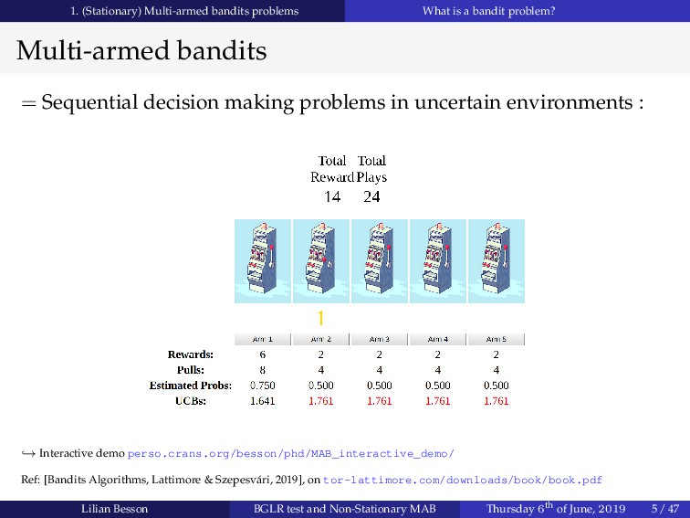
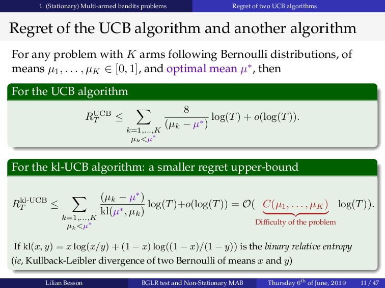
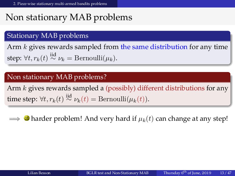
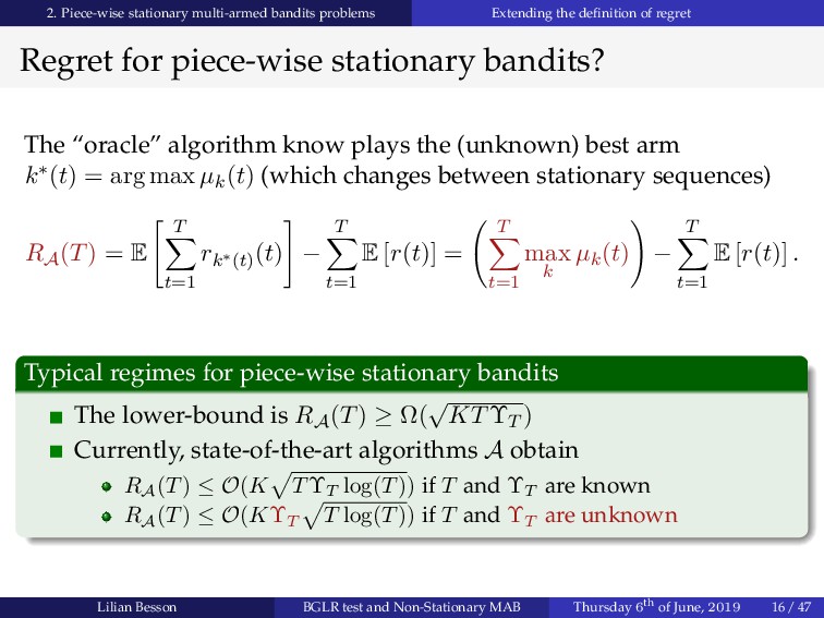
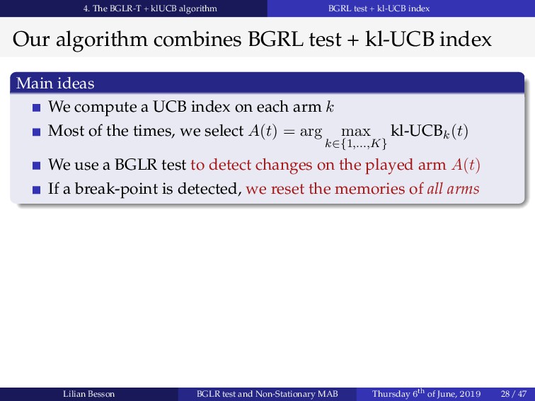
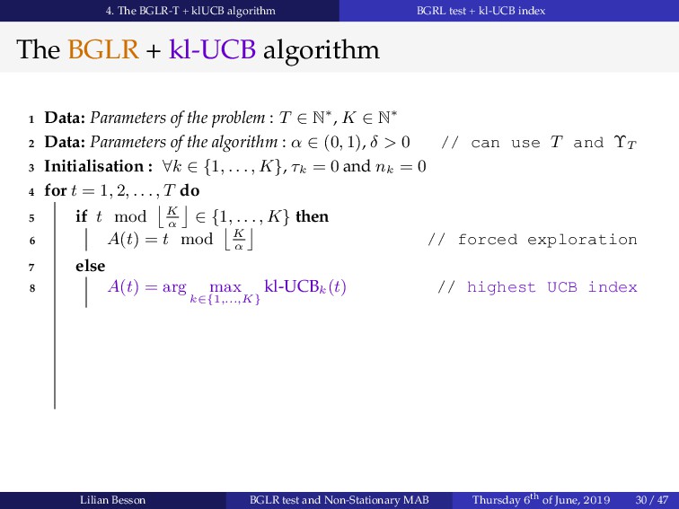
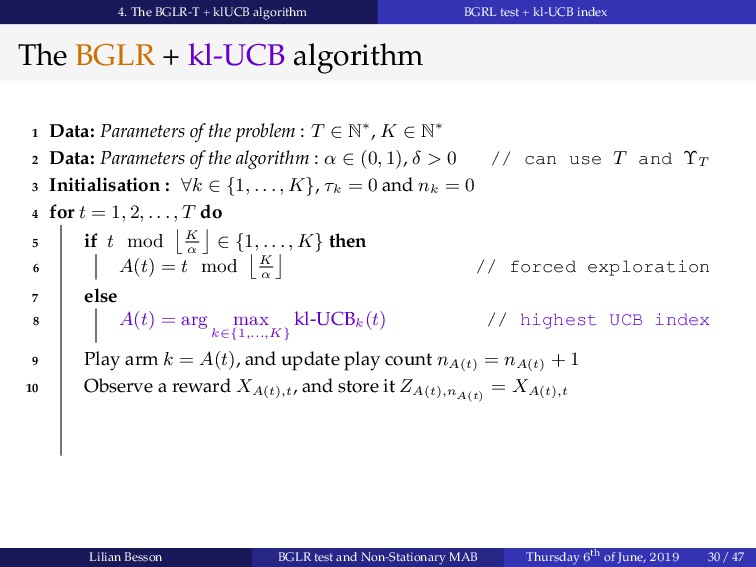
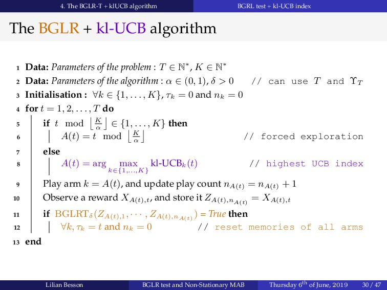
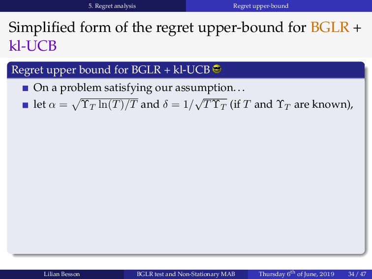
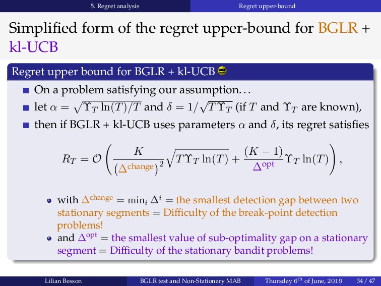
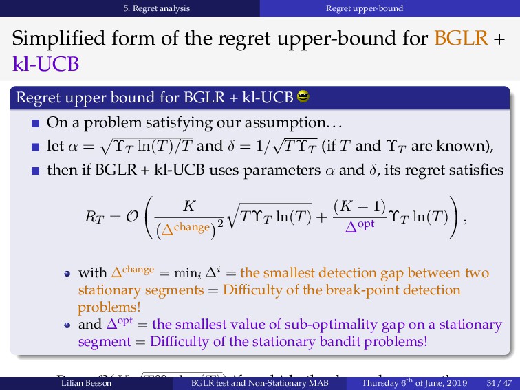
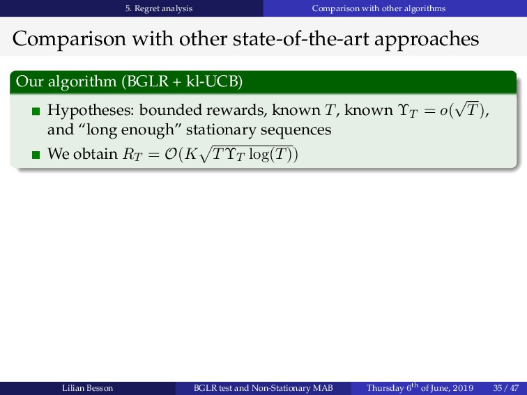
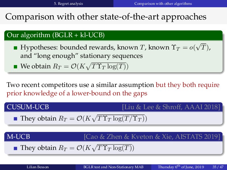
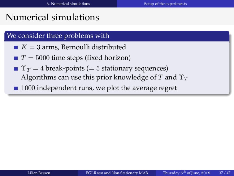
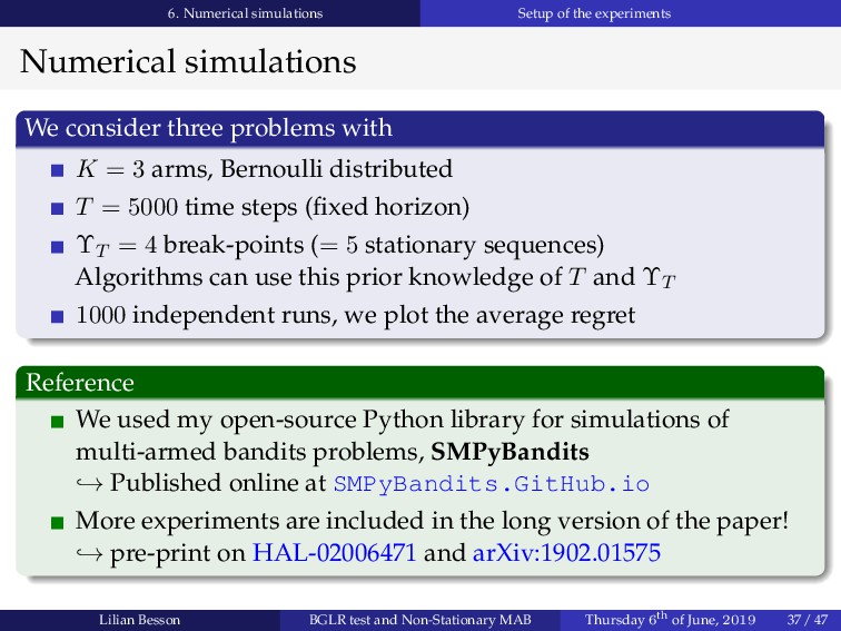
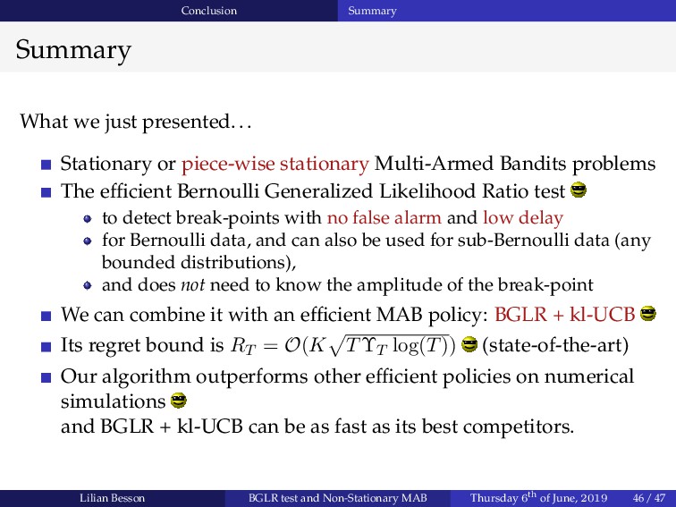
Abstract : We propose a new algorithm for the piece-wise i.i.d. non-stationary bandit problem with bounded rewards. Our proposal, GLR-klUCB, combines an efficient bandit algorithm, klUCB, with an efficient, parameter-free, change-point detector, the Bernoulli Generalized Likelihood Ratio Test, for which we provide new theoretical guarantees of independent interest. We analyze two variants of our strategy, based on local restarts and global restarts, and show that their regret is upper-bounded by O(Υ_T √(T log(T))) if the number of change-points Υ_T is unknown, and by O(√(Υ_T T log(T))) if Υ_T is known. This matches the current state-of-the-art bounds, as our algorithm needs no tuning based on knowledge of the problem complexity other than Υ_T. We present numerical experiments showing that GLR-klUCB outperforms passively and actively adaptive algorithms from the literature, and highlight the benefit of using local restarts.

See : https://hal.inria.fr/hal-02006471/
Format : 4:3

PDF: https://perso.crans.org/besson/slides/2019_06__About_Bernoulli_GLRTest__Seminar_at_PANAMA_IRISA_Rennes/slides.pdf

Transcript

1. The Bernoulli Generalized Likelihood Ratio test (BGLR) for Non-Stationary Multi-Armed Bandits Research Seminar at PANAMA, IRISA lab, Rennes Lilian Besson PhD Student SCEE team, IETR laboratory, CentraleSupélec in Rennes & SequeL team, CRIStAL laboratory, Inria in Lille Thursday 6th of June, 2019
2. Publications associated with this talk Joint work with my advisor Émilie Kaufmann : “Analyse non asymptotique d’un test séquentiel de détection de ruptures et application aux bandits non stationnaires” by Lilian Besson & Émilie Kaufmann → presented at GRETSI, in Lille (France), next August 2019 → perso.crans.org/besson/articles/BK__GRETSI_2019.pdf “The Generalized Likelihood Ratio Test meets klUCB: an Improved Algorithm for Piece-Wise Non-Stationary Bandits” by Lilian Besson & Émilie Kaufmann Pre-print on HAL-02006471 and arXiv:1902.01575 Lilian Besson BGLR test and Non-Stationary MAB Thursday 6th of June, 2019 2 / 47
3. Outline of the talk Outline of the talk 1 (Stationary) Multi-armed bandits problems 2 Piece-wise stationary multi-armed bandits problems 3 The BGLR test and its finite time properties 4 The BGLR-T + klUCB algorithm 5 Regret analysis 6 Numerical simulations Lilian Besson BGLR test and Non-Stationary MAB Thursday 6th of June, 2019 3 / 47
4. 1. (Stationary) Multi-armed bandits problems 1. (Stationary) Multi-armed bandits problems 1 (Stationary) Multi-armed bandits problems 2 Piece-wise stationary multi-armed bandits problems 3 The BGLR test and its finite time properties 4 The BGLR-T + klUCB algorithm 5 Regret analysis 6 Numerical simulations Lilian Besson BGLR test and Non-Stationary MAB Thursday 6th of June, 2019 4 / 47
5. 1. (Stationary) Multi-armed bandits problems What is a bandit problem? Multi-armed bandits = Sequential decision making problems in uncertain environments : → Interactive demo perso.crans.org/besson/phd/MAB_interactive_demo/ Ref: [Bandits Algorithms, Lattimore & Szepesvári, 2019], on tor-lattimore.com/downloads/book/book.pdf Lilian Besson BGLR test and Non-Stationary MAB Thursday 6th of June, 2019 5 / 47
6. 1. (Stationary) Multi-armed bandits problems Mathematical model Mathematical model Discrete time steps t = 1, . . . , T The horizon T is fixed and usually unknown At time t, an agent plays the arm A(t) ∈ {1, . . . , K}, then she observes the iid random reward r(t) ∼ νk, r(t) ∈ R Lilian Besson BGLR test and Non-Stationary MAB Thursday 6th of June, 2019 6 / 47
7. 1. (Stationary) Multi-armed bandits problems Mathematical model Mathematical model Discrete time steps t = 1, . . . , T The horizon T is fixed and usually unknown At time t, an agent plays the arm A(t) ∈ {1, . . . , K}, then she observes the iid random reward r(t) ∼ νk, r(t) ∈ R Usually, we focus on Bernoulli arms νk = Bernoulli(µk), of mean µk ∈ [0, 1], giving binary rewards r(t) ∈ {0, 1}. Lilian Besson BGLR test and Non-Stationary MAB Thursday 6th of June, 2019 6 / 47
8. 1. (Stationary) Multi-armed bandits problems Mathematical model Mathematical model Discrete time steps t = 1, . . . , T The horizon T is fixed and usually unknown At time t, an agent plays the arm A(t) ∈ {1, . . . , K}, then she observes the iid random reward r(t) ∼ νk, r(t) ∈ R Usually, we focus on Bernoulli arms νk = Bernoulli(µk), of mean µk ∈ [0, 1], giving binary rewards r(t) ∈ {0, 1}. Goal : maximize the sum of rewards T t=1 r(t) or maximize the sum of expected rewards E T t=1 r(t) Lilian Besson BGLR test and Non-Stationary MAB Thursday 6th of June, 2019 6 / 47
9. 1. (Stationary) Multi-armed bandits problems Mathematical model Mathematical model Discrete time steps t = 1, . . . , T The horizon T is fixed and usually unknown At time t, an agent plays the arm A(t) ∈ {1, . . . , K}, then she observes the iid random reward r(t) ∼ νk, r(t) ∈ R Usually, we focus on Bernoulli arms νk = Bernoulli(µk), of mean µk ∈ [0, 1], giving binary rewards r(t) ∈ {0, 1}. Goal : maximize the sum of rewards T t=1 r(t) or maximize the sum of expected rewards E T t=1 r(t) Any efficient policy must balance between exploration and exploitation: explore all arms to discover the best one, while exploiting the arms known to be good so far. Lilian Besson BGLR test and Non-Stationary MAB Thursday 6th of June, 2019 6 / 47
10. 1. (Stationary) Multi-armed bandits problems Naive solutions Two examples of bad solutions i) Pure exploration Play arm A(t) ∼ U({1, . . . , K}) uniformly at random =⇒ Mean expected rewards 1 T E T t=1 r(t) = 1 K K k=1 µk maxk µk Lilian Besson BGLR test and Non-Stationary MAB Thursday 6th of June, 2019 7 / 47
11. 1. (Stationary) Multi-armed bandits problems Naive solutions Two examples of bad solutions i) Pure exploration Play arm A(t) ∼ U({1, . . . , K}) uniformly at random =⇒ Mean expected rewards 1 T E T t=1 r(t) = 1 K K k=1 µk maxk µk ii) Pure exploitation Count the number of samples and the sum of rewards of each arm Nk(t) = s<t 1(A(s) = k) and Xk(t) = s<t r(s)1(A(s) = k) Estimate the unknown mean µk with µk(t) = Xk(t)/Nk(t) Play the arm of maximum empirical mean : A(t) = arg maxk µk(t) Performance depends on the first draws, and can be very poor! → Interactive demo perso.crans.org/besson/phd/MAB_interactive_demo/ Lilian Besson BGLR test and Non-Stationary MAB Thursday 6th of June, 2019 7 / 47
12. 1. (Stationary) Multi-armed bandits problems The “Upper Confidence Bound” algorithm A first solution: “Upper Confidence Bound” algorithm Compute UCBk(t) = Xk(t)/Nk(t) + α log(t)/Nk(t) = an upper confidence bound on the unknown mean µk Play the arm of maximal UCB : A(t) = arg maxk UCBk(t) → Principle of “optimism under uncertainty” α balances between exploitation (α → 0) and exploration (α → ∞) Lilian Besson BGLR test and Non-Stationary MAB Thursday 6th of June, 2019 8 / 47
13. 1. (Stationary) Multi-armed bandits problems The “Upper Confidence Bound” algorithm A first solution: “Upper Confidence Bound” algorithm Compute UCBk(t) = Xk(t)/Nk(t) + α log(t)/Nk(t) = an upper confidence bound on the unknown mean µk Play the arm of maximal UCB : A(t) = arg maxk UCBk(t) → Principle of “optimism under uncertainty” α balances between exploitation (α → 0) and exploration (α → ∞) UCB is efficient: the best arm is identified correctly (with high probability) if there are enough samples (for T large enough) =⇒ Expected rewards attains the maximum For T → ∞, 1 T E T t=1 r(t) → max k µk Lilian Besson BGLR test and Non-Stationary MAB Thursday 6th of June, 2019 8 / 47
14. 1. (Stationary) Multi-armed bandits problems The “Upper Confidence Bound” algorithm Elements of the proof for UCB algorithm Elements of proof of convergence (for K Bernoulli arms) Suppose the first arm is the best: µ∗ = µ1 > µ2 ≥ . . . ≥ µK Lilian Besson BGLR test and Non-Stationary MAB Thursday 6th of June, 2019 9 / 47
15. 1. (Stationary) Multi-armed bandits problems The “Upper Confidence Bound” algorithm Elements of the proof for UCB algorithm Elements of proof of convergence (for K Bernoulli arms) Suppose the first arm is the best: µ∗ = µ1 > µ2 ≥ . . . ≥ µK UCBk(t) = Xk(t)/Nk(t) + α log(t)/Nk(t) Lilian Besson BGLR test and Non-Stationary MAB Thursday 6th of June, 2019 9 / 47
16. 1. (Stationary) Multi-armed bandits problems The “Upper Confidence Bound” algorithm Elements of the proof for UCB algorithm Elements of proof of convergence (for K Bernoulli arms) Suppose the first arm is the best: µ∗ = µ1 > µ2 ≥ . . . ≥ µK UCBk(t) = Xk(t)/Nk(t) + α log(t)/Nk(t) Hoeffding’s inequality gives P(UCBk(t) < µk(t)) ≤ O( 1 t2α ) =⇒ the different UCBk(t) are true “Upper Confidence Bounds” on the (unknown) µk (most of the times) Lilian Besson BGLR test and Non-Stationary MAB Thursday 6th of June, 2019 9 / 47
17. 1. (Stationary) Multi-armed bandits problems The “Upper Confidence Bound” algorithm Elements of the proof for UCB algorithm Elements of proof of convergence (for K Bernoulli arms) Suppose the first arm is the best: µ∗ = µ1 > µ2 ≥ . . . ≥ µK UCBk(t) = Xk(t)/Nk(t) + α log(t)/Nk(t) Hoeffding’s inequality gives P(UCBk(t) < µk(t)) ≤ O( 1 t2α ) =⇒ the different UCBk(t) are true “Upper Confidence Bounds” on the (unknown) µk (most of the times) And if a suboptimal arm k > 1 is sampled, it implies UCBk(t) > UCB1(t), but µk < µ1: Hoeffding’s inequality also proves that any “wrong ordering” of the UCBk(t) is unlikely Lilian Besson BGLR test and Non-Stationary MAB Thursday 6th of June, 2019 9 / 47
18. 1. (Stationary) Multi-armed bandits problems The “Upper Confidence Bound” algorithm Elements of the proof for UCB algorithm Elements of proof of convergence (for K Bernoulli arms) Suppose the first arm is the best: µ∗ = µ1 > µ2 ≥ . . . ≥ µK UCBk(t) = Xk(t)/Nk(t) + α log(t)/Nk(t) Hoeffding’s inequality gives P(UCBk(t) < µk(t)) ≤ O( 1 t2α ) =⇒ the different UCBk(t) are true “Upper Confidence Bounds” on the (unknown) µk (most of the times) And if a suboptimal arm k > 1 is sampled, it implies UCBk(t) > UCB1(t), but µk < µ1: Hoeffding’s inequality also proves that any “wrong ordering” of the UCBk(t) is unlikely We can prove that suboptimal arms k are sampled about o(T) times =⇒ E T t=1 r(t) → T→∞ µ∗ × O(T) + k:∆k>0 µk × o(T) But... at which speed do we have this convergence? Lilian Besson BGLR test and Non-Stationary MAB Thursday 6th of June, 2019 9 / 47
19. 1. (Stationary) Multi-armed bandits problems Regret of a bandit algorithm Measure the performance of algorithm A by its mean regret RA (T) Difference in the accumulated rewards between an “oracle” and A The “oracle” algorithm always plays the (unknown) best arm k∗ = arg maxk µk (we note the best mean µk∗ = µ∗) Maximize the sum of expected rewards ⇐⇒ minimize the regret RA(T) = E T t=1 rk∗ (t) − T t=1 E [r(t)] = Tµ∗ − T t=1 E [r(t)] . Lilian Besson BGLR test and Non-Stationary MAB Thursday 6th of June, 2019 10 / 47
20. 1. (Stationary) Multi-armed bandits problems Regret of a bandit algorithm Measure the performance of algorithm A by its mean regret RA (T) Difference in the accumulated rewards between an “oracle” and A The “oracle” algorithm always plays the (unknown) best arm k∗ = arg maxk µk (we note the best mean µk∗ = µ∗) Maximize the sum of expected rewards ⇐⇒ minimize the regret RA(T) = E T t=1 rk∗ (t) − T t=1 E [r(t)] = Tµ∗ − T t=1 E [r(t)] . Typical regime for stationary bandits (lower & upper bounds) No algorithm A can obtain a regret better than RA(T) ≥ Ω(log(T)) And an efficient algorithm A obtains RA(T) ≤ O(log(T)) Lilian Besson BGLR test and Non-Stationary MAB Thursday 6th of June, 2019 10 / 47
21. 1. (Stationary) Multi-armed bandits problems Regret of two UCB algorithms Regret of the UCB algorithm and another algorithm For any problem with K arms following Bernoulli distributions, of means µ1, . . . , µK ∈ [0, 1], and optimal mean µ∗, then For the UCB algorithm RUCB T ≤ k=1,...,K µk<µ∗ 8 (µk − µ∗) log(T) + o(log(T)). Lilian Besson BGLR test and Non-Stationary MAB Thursday 6th of June, 2019 11 / 47
22. 1. (Stationary) Multi-armed bandits problems Regret of two UCB algorithms Regret of the UCB algorithm and another algorithm For any problem with K arms following Bernoulli distributions, of means µ1, . . . , µK ∈ [0, 1], and optimal mean µ∗, then For the UCB algorithm RUCB T ≤ k=1,...,K µk<µ∗ 8 (µk − µ∗) log(T) + o(log(T)). For the kl-UCB algorithm: a smaller regret upper-bound Rkl-UCB T ≤ k=1,...,K µk<µ∗ (µk − µ∗) kl(µ∗, µk ) log(T)+o(log(T)) = O( C(µ1 , . . . , µK ) Difficulty of the problem log(T)). If kl(x, y) = x log(x/y) + (1 − x) log((1 − x)/(1 − y)) is the binary relative entropy (ie, Kullback-Leibler divergence of two Bernoulli of means x and y) Lilian Besson BGLR test and Non-Stationary MAB Thursday 6th of June, 2019 11 / 47
23. 2. Piece-wise stationary multi-armed bandits problems 2. Piece-wise stationary MAB problems 1 (Stationary) Multi-armed bandits problems 2 Piece-wise stationary multi-armed bandits problems 3 The BGLR test and its finite time properties 4 The BGLR-T + klUCB algorithm 5 Regret analysis 6 Numerical simulations Lilian Besson BGLR test and Non-Stationary MAB Thursday 6th of June, 2019 12 / 47
24. 2. Piece-wise stationary multi-armed bandits problems Non stationary MAB problems Stationary MAB problems Arm k gives rewards sampled from the same distribution for any time step: ∀t, rk(t) iid ∼ νk = Bernoulli(µk). Lilian Besson BGLR test and Non-Stationary MAB Thursday 6th of June, 2019 13 / 47
25. 2. Piece-wise stationary multi-armed bandits problems Non stationary MAB problems Stationary MAB problems Arm k gives rewards sampled from the same distribution for any time step: ∀t, rk(t) iid ∼ νk = Bernoulli(µk). Non stationary MAB problems? Arm k gives rewards sampled a (possibly) different distributions for any time step: ∀t, rk(t) iid ∼ νk(t) = Bernoulli(µk(t)). =⇒ harder problem! And very hard if µk(t) can change at any step! Lilian Besson BGLR test and Non-Stationary MAB Thursday 6th of June, 2019 13 / 47
26. 2. Piece-wise stationary multi-armed bandits problems Non stationary MAB problems Stationary MAB problems Arm k gives rewards sampled from the same distribution for any time step: ∀t, rk(t) iid ∼ νk = Bernoulli(µk). Non stationary MAB problems? Arm k gives rewards sampled a (possibly) different distributions for any time step: ∀t, rk(t) iid ∼ νk(t) = Bernoulli(µk(t)). =⇒ harder problem! And very hard if µk(t) can change at any step! Piece-wise stationary problems! → we focus on the easier case when there are at most o( √ T) intervals on which the means are all stationary (= sequence) Lilian Besson BGLR test and Non-Stationary MAB Thursday 6th of June, 2019 13 / 47
27. 2. Piece-wise stationary multi-armed bandits problems Definitions Break-points and stationary sequences Define The number of break-points ΥT = T−1 t=1 1(∃k ∈ {1, . . . , K} : µk(t) = µk(t + 1)) The i-th break-point τi = inf{t > τi−1 : ∃k : µk(t) = µk(t + 1)} (with τ0 = 0) Lilian Besson BGLR test and Non-Stationary MAB Thursday 6th of June, 2019 14 / 47
28. 2. Piece-wise stationary multi-armed bandits problems Definitions Break-points and stationary sequences Define The number of break-points ΥT = T−1 t=1 1(∃k ∈ {1, . . . , K} : µk(t) = µk(t + 1)) The i-th break-point τi = inf{t > τi−1 : ∃k : µk(t) = µk(t + 1)} (with τ0 = 0) Hypotheses on piece-wise stationary problems The rewards rk(t) generated by each arm k are iid on each interval [τi + 1, τi+1] (the i-th sequence) There are ΥT = o( √ T) break-points And ΥT can be known before-hand All sequences are “long enough” Lilian Besson BGLR test and Non-Stationary MAB Thursday 6th of June, 2019 14 / 47
29. Example of a piece-wise stationary MAB problem We plots the means µ1(t), µ2(t), µ3(t) of K = 3 arms. There are ΥT = 4 break-points and 5 sequences between t = 1 and t = T = 5000: 0 1000 2000 3000 4000 5000 Time steps t=1...T, horizon T=5000 0.2 0.4 0.6 0.8 Successive means of the K=3 arms History of means for Non-Stationary MAB, Bernoulli with 4 break-points Arm #0 Arm #1 Arm #2
30. 2. Piece-wise stationary multi-armed bandits problems Extending the definition of regret Regret for piece-wise stationary bandits? The “oracle” algorithm know plays the (unknown) best arm k∗(t) = arg max µk(t) (which changes between stationary sequences) RA(T) = E T t=1 rk∗(t) (t) − T t=1 E [r(t)] = T t=1 max k µk(t) − T t=1 E [r(t)] . Lilian Besson BGLR test and Non-Stationary MAB Thursday 6th of June, 2019 16 / 47
31. 2. Piece-wise stationary multi-armed bandits problems Extending the definition of regret Regret for piece-wise stationary bandits? The “oracle” algorithm know plays the (unknown) best arm k∗(t) = arg max µk(t) (which changes between stationary sequences) RA(T) = E T t=1 rk∗(t) (t) − T t=1 E [r(t)] = T t=1 max k µk(t) − T t=1 E [r(t)] . Typical regimes for piece-wise stationary bandits The lower-bound is RA(T) ≥ Ω( √ KTΥT ) Currently, state-of-the-art algorithms A obtain RA (T) ≤ O(K TΥT log(T)) if T and ΥT are known RA (T) ≤ O(KΥT T log(T)) if T and ΥT are unknown Lilian Besson BGLR test and Non-Stationary MAB Thursday 6th of June, 2019 16 / 47
32. 3. The BGLR test and its finite time properties 3. The BGLR test and its finite time properties 1 (Stationary) Multi-armed bandits problems 2 Piece-wise stationary multi-armed bandits problems 3 The BGLR test and its finite time properties 4 The BGLR-T + klUCB algorithm 5 Regret analysis 6 Numerical simulations Lilian Besson BGLR test and Non-Stationary MAB Thursday 6th of June, 2019 17 / 47
33. 3. The BGLR test and its finite time properties Break-point detection The break-point detection problem Imagine the following problem. . . You observe data X1, X2, · · · , Xt, · · · ∈ [0, 1] sequentially. . . You know that Xt is generated by a certain unknown distribution... Lilian Besson BGLR test and Non-Stationary MAB Thursday 6th of June, 2019 18 / 47
34. 3. The BGLR test and its finite time properties Break-point detection The break-point detection problem Imagine the following problem. . . You observe data X1, X2, · · · , Xt, · · · ∈ [0, 1] sequentially. . . You know that Xt is generated by a certain unknown distribution... Your goal is to distinguish between two hypotheses: H0 The distributions all have the same mean (“no break-point”) ∃µ0 , E[X1 ] = E[X2 ] = · · · = E[Xt ] = µ0 H1 The distributions have changed mean at a break-point at time τ ∃µ0 , µ1 , τ, E[X1 ] = · · · = E[Xτ ] = µ0 , µ0 = µ1 , E[Xτ+1 ] = E[Xτ+2 ] = · · · = µ1 You stop at time τ, as soon as you detect a change Lilian Besson BGLR test and Non-Stationary MAB Thursday 6th of June, 2019 18 / 47
35. 3. The BGLR test and its finite time properties Break-point detection The break-point detection problem Imagine the following problem. . . You observe data X1, X2, · · · , Xt, · · · ∈ [0, 1] sequentially. . . You know that Xt is generated by a certain unknown distribution... Your goal is to distinguish between two hypotheses: H0 The distributions all have the same mean (“no break-point”) ∃µ0 , E[X1 ] = E[X2 ] = · · · = E[Xt ] = µ0 H1 The distributions have changed mean at a break-point at time τ ∃µ0 , µ1 , τ, E[X1 ] = · · · = E[Xτ ] = µ0 , µ0 = µ1 , E[Xτ+1 ] = E[Xτ+2 ] = · · · = µ1 You stop at time τ, as soon as you detect a change A sequential break-point detection is a stopping time τ, measurable for Ft = σ(X1, · · · , Xt), which rejects hypothesis H0 when τ < ∞. Lilian Besson BGLR test and Non-Stationary MAB Thursday 6th of June, 2019 18 / 47
36. 3. The BGLR test and its finite time properties Likelihood ratio test for Bernoulli observations Bernoulli likelihood ratio test Hypothesis: all distributions are Bernoulli The problem boils down to distinguishing H0: (∃µ0 : ∀i ∈ N∗, Xi i.i.d. ∼ (µ0)), against the alternative H1: (∃µ0 = µ1, τ > 1 : X1, · · · , Xτ i.i.d. ∼ (µ0) et Xτ+1, · · · i.i.d. ∼ (µ1)). Lilian Besson BGLR test and Non-Stationary MAB Thursday 6th of June, 2019 19 / 47
37. 3. The BGLR test and its finite time properties Likelihood ratio test for Bernoulli observations Bernoulli likelihood ratio test Hypothesis: all distributions are Bernoulli The problem boils down to distinguishing H0: (∃µ0 : ∀i ∈ N∗, Xi i.i.d. ∼ (µ0)), against the alternative H1: (∃µ0 = µ1, τ > 1 : X1, · · · , Xτ i.i.d. ∼ (µ0) et Xτ+1, · · · i.i.d. ∼ (µ1)). The Likelihood Ratio statistic for this hypothesis test, after observing X1, · · · , Xn, is L(n) = sup µ0,µ1,τ<n (X1 , · · · , Xn ; µ0 , µ1 , τ) sup µ0 (X1 , · · · , Xn ; µ0 ) , where (X1, · · · , Xn; µ0) (resp. (X1, · · · , Xn; µ0, µ1, τ)) is the likelihood of the observations under a model in H0 (resp. H1). Lilian Besson BGLR test and Non-Stationary MAB Thursday 6th of June, 2019 19 / 47
38. 3. The BGLR test and its finite time properties Likelihood ratio test for Bernoulli observations Bernoulli likelihood ratio test Hypothesis: all distributions are Bernoulli The problem boils down to distinguishing H0: (∃µ0 : ∀i ∈ N∗, Xi i.i.d. ∼ (µ0)), against the alternative H1: (∃µ0 = µ1, τ > 1 : X1, · · · , Xτ i.i.d. ∼ (µ0) et Xτ+1, · · · i.i.d. ∼ (µ1)). The Likelihood Ratio statistic for this hypothesis test, after observing X1, · · · , Xn, is L(n) = sup µ0,µ1,τ<n (X1 , · · · , Xn ; µ0 , µ1 , τ) sup µ0 (X1 , · · · , Xn ; µ0 ) , where (X1, · · · , Xn; µ0) (resp. (X1, · · · , Xn; µ0, µ1, τ)) is the likelihood of the observations under a model in H0 (resp. H1). → High values of this statistic L(n) tends to reject H0 over H1. Lilian Besson BGLR test and Non-Stationary MAB Thursday 6th of June, 2019 19 / 47
39. 3. The BGLR test and its finite time properties Likelihood ratio test for Bernoulli observations Expression of the (log) Bernoulli Likelihood ratio We can rewrite this statistic L(n) = sup µ0,µ1,τ<n (X1,··· ,Xn;µ0,µ1,τ) sup µ0 (X1,··· ,Xn;µ0) , by using Bernoulli likelihood, and shifting means µk:k = 1 k −k+1 k s=k Xs : log L(n) = max s∈{2,··· ,n−1} s × kl( µ1:s before change , µ1:n all data ) +(n − s) × kl( µs+1:n after change , µ1:n all data ) . Where kl(x, y) = x ln x/y + (1 − x) ln (1 − x)/(1 − y) is the binary relative entropy Lilian Besson BGLR test and Non-Stationary MAB Thursday 6th of June, 2019 20 / 47
40. 3. The BGLR test and its finite time properties The BGLR-T The Bernoulli Generalized likelihood ratio test (BGLR) We can extend the Bernoulli likelihood ratio test if the observations are sub-Bernoulli. And any bounded distributions on [0, 1] is sub-Bernoulli ! =⇒ the BGLR test can be applied for any bounded observations Lilian Besson BGLR test and Non-Stationary MAB Thursday 6th of June, 2019 21 / 47
41. 3. The BGLR test and its finite time properties The BGLR-T The Bernoulli Generalized likelihood ratio test (BGLR) We can extend the Bernoulli likelihood ratio test if the observations are sub-Bernoulli. And any bounded distributions on [0, 1] is sub-Bernoulli ! =⇒ the BGLR test can be applied for any bounded observations The BGRL-T sequential break-point detection test The BGLR-T is the stopping time defined by τδ = inf n ∈ N∗ : max s∈{2,··· ,n−1} s kl (µ1:s , µ1:n )+(n−s) kl (µs+1:n , µ1:n ) ≥ β(n, δ) with a threshold function β(n, δ) specified later, n is the number of observations, δ is the confidence level. Lilian Besson BGLR test and Non-Stationary MAB Thursday 6th of June, 2019 21 / 47
42. 3. The BGLR test and its finite time properties False alarm Probability of false alarm A good test should not detect any break-point if there is no break-point to detect... Lilian Besson BGLR test and Non-Stationary MAB Thursday 6th of June, 2019 22 / 47
43. 3. The BGLR test and its finite time properties False alarm Probability of false alarm A good test should not detect any break-point if there is no break-point to detect... Definition: False alarm The stopping time is τδ, and a break-point is detected if τδ < ∞. Let Pµ0 be a probability model under which the observations are ∀t, Xt ∈ [0, 1] and ∀t, E[Xt] = µ0. The false alarm probability is Pµ0 (τδ < ∞). =⇒ Goal: controlling the false alarm event! (in high probability) Lilian Besson BGLR test and Non-Stationary MAB Thursday 6th of June, 2019 22 / 47
44. 3. The BGLR test and its finite time properties False alarm First result for the BGLR test Controlling the false alarm probability For any confidence level 0 < δ < 1, the BGLR test satisfies Pµ0 (τδ < ∞) ≤ δ with the threshold function β(n, δ) = 2 T ln(3n √ n/δ) 2 + 6 ln(1 + ln(n)) ln 3n √ n δ = O log n δ . Where T (x) verifies T (x) x + ln(x) for x large enough Lilian Besson BGLR test and Non-Stationary MAB Thursday 6th of June, 2019 23 / 47
45. 3. The BGLR test and its finite time properties False alarm First result for the BGLR test Controlling the false alarm probability For any confidence level 0 < δ < 1, the BGLR test satisfies Pµ0 (τδ < ∞) ≤ δ with the threshold function β(n, δ) = 2 T ln(3n √ n/δ) 2 + 6 ln(1 + ln(n)) ln 3n √ n δ = O log n δ . Where T (x) verifies T (x) x + ln(x) for x large enough Proof ? Hard to explain in a short time. . . → see the article, on HAL-02006471 and arXiv:1902.01575 Lilian Besson BGLR test and Non-Stationary MAB Thursday 6th of June, 2019 23 / 47
46. 3. The BGLR test and its finite time properties Delay of detection Delay of detection A good test should detect a break-point “fast enough” if there is a break-point to detect, with enough samples before the break-point. . . Lilian Besson BGLR test and Non-Stationary MAB Thursday 6th of June, 2019 24 / 47
47. 3. The BGLR test and its finite time properties Delay of detection Delay of detection A good test should detect a break-point “fast enough” if there is a break-point to detect, with enough samples before the break-point. . . Definition: Delay of detection Let Pµ0,µ1,τ be a probability model under which ∀t, Xt ∈ [0, 1] and ∀t ≤ τ, E[Xt] = µ0 and ∀t ≥ τ + 1, E[Xt] = µ1, with µ0 = µ1. The gap of this break-point is ∆ = |µ0 − µ1|. The delay of detection is u = τδ − τ ∈ N. =⇒ Goal: controlling the delay of detection! (in high probability) Lilian Besson BGLR test and Non-Stationary MAB Thursday 6th of June, 2019 24 / 47
48. 3. The BGLR test and its finite time properties Delay of detection Second result for the BGLR test Controlling the delay of detection On a break-point of amplitude ∆ = |µ1 − µ0|, the BGLRT test satisfies Pµ0,µ1,τ (τδ ≥ τ + u) ≤ exp  − 2τu τ + u max 0, ∆ − τ + u 2τu β(τ + u, δ) 2  = O(exp (u)). with the same threshold function β(n, δ) ln(3n √ n/δ). Consequence In high probability, the delay τδ of BGLR is bounded by O(∆−2 ln(1/δ)) if enough samples are observed before the break-point at time τ. Lilian Besson BGLR test and Non-Stationary MAB Thursday 6th of June, 2019 25 / 47
49. 3. The BGLR test and its finite time properties Summary of results for BGLR-T BGLR is an efficient break-point detection test ! We just saw that by choosing a confidence level δ, and a good threshold function β(n, δ) ln(3n √ n/δ) = O(log(n/δ)) Lilian Besson BGLR test and Non-Stationary MAB Thursday 6th of June, 2019 26 / 47
50. 3. The BGLR test and its finite time properties Summary of results for BGLR-T BGLR is an efficient break-point detection test ! We just saw that by choosing a confidence level δ, and a good threshold function β(n, δ) ln(3n √ n/δ) = O(log(n/δ)) we can control the two properties of the BGLR test: its false alarm probability: Pµ0 (τδ < ∞) ≤ δ its detection delay: Pµ0,µ1,τ (τδ ≥ τ + u) decreases exponentially fast wrt u (if there are enough samples before and after the break-point) =⇒ The BGLR is an efficient break-point detection test Lilian Besson BGLR test and Non-Stationary MAB Thursday 6th of June, 2019 26 / 47
51. 3. The BGLR test and its finite time properties Summary of results for BGLR-T BGLR is an efficient break-point detection test ! We just saw that by choosing a confidence level δ, and a good threshold function β(n, δ) ln(3n √ n/δ) = O(log(n/δ)) we can control the two properties of the BGLR test: its false alarm probability: Pµ0 (τδ < ∞) ≤ δ its detection delay: Pµ0,µ1,τ (τδ ≥ τ + u) decreases exponentially fast wrt u (if there are enough samples before and after the break-point) =⇒ The BGLR is an efficient break-point detection test Finite time guarantees [Maillard, ALT, 2019] [Lai & Xing, Sequential Analysis, 2010] Such finite time (non asymptotic) guarantees are recent results! Lilian Besson BGLR test and Non-Stationary MAB Thursday 6th of June, 2019 26 / 47
52. 4. The BGLR-T + klUCB algorithm 4. The BGLR-T + klUCB algorithm 1 (Stationary) Multi-armed bandits problems 2 Piece-wise stationary multi-armed bandits problems 3 The BGLR test and its finite time properties 4 The BGLR-T + klUCB algorithm 5 Regret analysis 6 Numerical simulations Lilian Besson BGLR test and Non-Stationary MAB Thursday 6th of June, 2019 27 / 47
53. 4. The BGLR-T + klUCB algorithm BGRL test + kl-UCB index Our algorithm combines BGRL test + kl-UCB index Main ideas We compute a UCB index on each arm k Most of the times, we select A(t) = arg max k∈{1,...,K} kl-UCBk(t) We use a BGLR test to detect changes on the played arm A(t) If a break-point is detected, we reset the memories of all arms Lilian Besson BGLR test and Non-Stationary MAB Thursday 6th of June, 2019 28 / 47
54. 4. The BGLR-T + klUCB algorithm BGRL test + kl-UCB index Our algorithm combines BGRL test + kl-UCB index Main ideas We compute a UCB index on each arm k Most of the times, we select A(t) = arg max k∈{1,...,K} kl-UCBk(t) We use a BGLR test to detect changes on the played arm A(t) If a break-point is detected, we reset the memories of all arms The kl-UCB indexes τk(t) is the time of last reset of arm k before time t, nk(t) counts the selections and µk(t) is the empirical means of observations of arm k since τk(t), Let kl-UCBk (t) = max q ∈ [0, 1] : nk (t) × kl (µk (t), q) ≤ f(t − τk (t)) f(t) = ln(t) + 3 ln(ln(t)) controls the width of the UCB. Lilian Besson BGLR test and Non-Stationary MAB Thursday 6th of June, 2019 28 / 47
55. 4. The BGLR-T + klUCB algorithm BGRL test + kl-UCB index Two details of our algorithm i) How do we use the BGLR test? (parameter δ) From observations Z1, · · · , Zn we detect a break-point with confidence level δ when sup 1<s<n s × kl Z1:s, Z1:n + (n − s) × kl Zs+1:n, Z1:n ≥ β(n, δ) Lilian Besson BGLR test and Non-Stationary MAB Thursday 6th of June, 2019 29 / 47
56. 4. The BGLR-T + klUCB algorithm BGRL test + kl-UCB index Two details of our algorithm i) How do we use the BGLR test? (parameter δ) From observations Z1, · · · , Zn we detect a break-point with confidence level δ when sup 1<s<n s × kl Z1:s, Z1:n + (n − s) × kl Zs+1:n, Z1:n ≥ β(n, δ) ii) Forced exploration (parameter α) We use a forced exploration uniformly on all arms. . . ie, in average, arm k is forced to be sampled at least T × α/K times =⇒ so we can detect break-points on all the arms and not only on the arm played by the kl-UCB indexes Lilian Besson BGLR test and Non-Stationary MAB Thursday 6th of June, 2019 29 / 47
57. 4. The BGLR-T + klUCB algorithm BGRL test + kl-UCB index The BGLR + kl-UCB algorithm 1 Data: Parameters of the problem : T ∈ N∗, K ∈ N∗ 2 Data: Parameters of the algorithm : α ∈ (0, 1), δ > 0 // can use T and ΥT 3 Initialisation : ∀k ∈ {1, . . . , K}, τk = 0 and nk = 0 4 for t = 1, 2, . . . , T do Lilian Besson BGLR test and Non-Stationary MAB Thursday 6th of June, 2019 30 / 47
58. 4. The BGLR-T + klUCB algorithm BGRL test + kl-UCB index The BGLR + kl-UCB algorithm 1 Data: Parameters of the problem : T ∈ N∗, K ∈ N∗ 2 Data: Parameters of the algorithm : α ∈ (0, 1), δ > 0 // can use T and ΥT 3 Initialisation : ∀k ∈ {1, . . . , K}, τk = 0 and nk = 0 4 for t = 1, 2, . . . , T do 5 if t mod K α ∈ {1, . . . , K} then 6 A(t) = t mod K α // forced exploration 7 else 8 A(t) = arg max k∈{1,...,K} kl-UCBk (t) // highest UCB index Lilian Besson BGLR test and Non-Stationary MAB Thursday 6th of June, 2019 30 / 47
59. 4. The BGLR-T + klUCB algorithm BGRL test + kl-UCB index The BGLR + kl-UCB algorithm 1 Data: Parameters of the problem : T ∈ N∗, K ∈ N∗ 2 Data: Parameters of the algorithm : α ∈ (0, 1), δ > 0 // can use T and ΥT 3 Initialisation : ∀k ∈ {1, . . . , K}, τk = 0 and nk = 0 4 for t = 1, 2, . . . , T do 5 if t mod K α ∈ {1, . . . , K} then 6 A(t) = t mod K α // forced exploration 7 else 8 A(t) = arg max k∈{1,...,K} kl-UCBk (t) // highest UCB index 9 Play arm k = A(t), and update play count nA(t) = nA(t) + 1 10 Observe a reward XA(t),t , and store it ZA(t),nA(t) = XA(t),t Lilian Besson BGLR test and Non-Stationary MAB Thursday 6th of June, 2019 30 / 47
60. 4. The BGLR-T + klUCB algorithm BGRL test + kl-UCB index The BGLR + kl-UCB algorithm 1 Data: Parameters of the problem : T ∈ N∗, K ∈ N∗ 2 Data: Parameters of the algorithm : α ∈ (0, 1), δ > 0 // can use T and ΥT 3 Initialisation : ∀k ∈ {1, . . . , K}, τk = 0 and nk = 0 4 for t = 1, 2, . . . , T do 5 if t mod K α ∈ {1, . . . , K} then 6 A(t) = t mod K α // forced exploration 7 else 8 A(t) = arg max k∈{1,...,K} kl-UCBk (t) // highest UCB index 9 Play arm k = A(t), and update play count nA(t) = nA(t) + 1 10 Observe a reward XA(t),t , and store it ZA(t),nA(t) = XA(t),t 11 if BGLRTδ (ZA(t),1 , · · · , ZA(t),nA(t) ) = True then 12 ∀k, τk = t and nk = 0 // reset memories of all arms 13 end Lilian Besson BGLR test and Non-Stationary MAB Thursday 6th of June, 2019 30 / 47
61. 5. Regret analysis 5. Regret analysis 1 (Stationary) Multi-armed bandits problems 2 Piece-wise stationary multi-armed bandits problems 3 The BGLR test and its finite time properties 4 The BGLR-T + klUCB algorithm 5 Regret analysis 6 Numerical simulations Lilian Besson BGLR test and Non-Stationary MAB Thursday 6th of June, 2019 31 / 47
62. 5. Regret analysis Hypotheses Hypotheses of our theoretical analysis Denote τi the position of break-point i (τ0 = 0) and µi k the mean of arm k on the segment [τi, τi+1] and b(i) ∈ arg maxk µi k (one of) the best arm(s) on the i-th segment and the largest gap at break-point i is ∆i = max k=1,...,K |µi k − µi−1 k | > 0 Lilian Besson BGLR test and Non-Stationary MAB Thursday 6th of June, 2019 32 / 47
63. 5. Regret analysis Hypotheses Hypotheses of our theoretical analysis Denote τi the position of break-point i (τ0 = 0) and µi k the mean of arm k on the segment [τi, τi+1] and b(i) ∈ arg maxk µi k (one of) the best arm(s) on the i-th segment and the largest gap at break-point i is ∆i = max k=1,...,K |µi k − µi−1 k | > 0 Assumption Fix the parameters α and δ, and let di = di(α, δ) = 4K α(∆i)2 β(T, δ) + K α . We assume that all sequences are “long enough”: ∀i ∈ {1, . . . , ΥT }, τi − τi−1 ≥ 2 max(di, di−1). Lilian Besson BGLR test and Non-Stationary MAB Thursday 6th of June, 2019 32 / 47
64. 5. Regret analysis Hypotheses Hypotheses of our theoretical analysis Denote τi the position of break-point i (τ0 = 0) and µi k the mean of arm k on the segment [τi, τi+1] and b(i) ∈ arg maxk µi k (one of) the best arm(s) on the i-th segment and the largest gap at break-point i is ∆i = max k=1,...,K |µi k − µi−1 k | > 0 Assumption Fix the parameters α and δ, and let di = di(α, δ) = 4K α(∆i)2 β(T, δ) + K α . We assume that all sequences are “long enough”: ∀i ∈ {1, . . . , ΥT }, τi − τi−1 ≥ 2 max(di, di−1). → The minimum length of sequence i depends on the amplitude of the changes at the beginning and the end of the sequence (∆i−1 and ∆i). Lilian Besson BGLR test and Non-Stationary MAB Thursday 6th of June, 2019 32 / 47
65. 5. Regret analysis Regret upper-bound Theoretical result Under this hypothesis, we obtained a finite time upper-bound on the regret RT , with explicit dependency from the problem difficulty. The exact bound uses: the divergences kl(µi k , µi b(i) ) account for the difficulty of the stationary problem on sequence i, the gaps ∆i account for the difficulty of detecting break-point i, as well as the two parameters α the probability of forced exploration, and δ the confidence level of the break-point detection test. Lilian Besson BGLR test and Non-Stationary MAB Thursday 6th of June, 2019 33 / 47
66. 5. Regret analysis Regret upper-bound Simplified form of the regret upper-bound for BGLR + kl-UCB Regret upper bound for BGLR + kl-UCB On a problem satisfying our assumption. . . let α = ΥT ln(T)/T and δ = 1/ √ TΥT (if T and ΥT are known), Lilian Besson BGLR test and Non-Stationary MAB Thursday 6th of June, 2019 34 / 47
67. 5. Regret analysis Regret upper-bound Simplified form of the regret upper-bound for BGLR + kl-UCB Regret upper bound for BGLR + kl-UCB On a problem satisfying our assumption. . . let α = ΥT ln(T)/T and δ = 1/ √ TΥT (if T and ΥT are known), then if BGLR + kl-UCB uses parameters α and δ, its regret satisfies RT = O K ∆change 2 TΥT ln(T) + (K − 1) ∆opt ΥT ln(T) , with ∆change = mini ∆i = the smallest detection gap between two stationary segments = Difficulty of the break-point detection problems! and ∆opt = the smallest value of sub-optimality gap on a stationary segment = Difficulty of the stationary bandit problems! Lilian Besson BGLR test and Non-Stationary MAB Thursday 6th of June, 2019 34 / 47
68. 5. Regret analysis Regret upper-bound Simplified form of the regret upper-bound for BGLR + kl-UCB Regret upper bound for BGLR + kl-UCB On a problem satisfying our assumption. . . let α = ΥT ln(T)/T and δ = 1/ √ TΥT (if T and ΥT are known), then if BGLR + kl-UCB uses parameters α and δ, its regret satisfies RT = O K ∆change 2 TΥT ln(T) + (K − 1) ∆opt ΥT ln(T) , with ∆change = mini ∆i = the smallest detection gap between two stationary segments = Difficulty of the break-point detection problems! and ∆opt = the smallest value of sub-optimality gap on a stationary segment = Difficulty of the stationary bandit problems! =⇒ RT = O(K TΥT log(T)) if we hide the dependency on the gaps. Lilian Besson BGLR test and Non-Stationary MAB Thursday 6th of June, 2019 34 / 47
69. 5. Regret analysis Comparison with other algorithms Comparison with other state-of-the-art approaches Our algorithm (BGLR + kl-UCB) Hypotheses: bounded rewards, known T, known ΥT = o( √ T), and “long enough” stationary sequences We obtain RT = O(K TΥT log(T)) Lilian Besson BGLR test and Non-Stationary MAB Thursday 6th of June, 2019 35 / 47
70. 5. Regret analysis Comparison with other algorithms Comparison with other state-of-the-art approaches Our algorithm (BGLR + kl-UCB) Hypotheses: bounded rewards, known T, known ΥT = o( √ T), and “long enough” stationary sequences We obtain RT = O(K TΥT log(T)) Two recent competitors use a similar assumption but they both require prior knowledge of a lower-bound on the gaps CUSUM-UCB [Liu & Lee & Shroff, AAAI 2018] They obtain RT = O(K TΥT log(T/ΥT )) M-UCB [Cao & Zhen & Kveton & Xie, AISTATS 2019] They obtain RT = O(K TΥT log(T)) Lilian Besson BGLR test and Non-Stationary MAB Thursday 6th of June, 2019 35 / 47
71. 6. Numerical simulations 6. Numerical simulations 1 (Stationary) Multi-armed bandits problems 2 Piece-wise stationary multi-armed bandits problems 3 The BGLR test and its finite time properties 4 The BGLR-T + klUCB algorithm 5 Regret analysis 6 Numerical simulations Lilian Besson BGLR test and Non-Stationary MAB Thursday 6th of June, 2019 36 / 47
72. 6. Numerical simulations Setup of the experiments Numerical simulations We consider three problems with K = 3 arms, Bernoulli distributed T = 5000 time steps (fixed horizon) ΥT = 4 break-points (= 5 stationary sequences) Algorithms can use this prior knowledge of T and ΥT 1000 independent runs, we plot the average regret Lilian Besson BGLR test and Non-Stationary MAB Thursday 6th of June, 2019 37 / 47
73. 6. Numerical simulations Setup of the experiments Numerical simulations We consider three problems with K = 3 arms, Bernoulli distributed T = 5000 time steps (fixed horizon) ΥT = 4 break-points (= 5 stationary sequences) Algorithms can use this prior knowledge of T and ΥT 1000 independent runs, we plot the average regret Reference We used my open-source Python library for simulations of multi-armed bandits problems, SMPyBandits → Published online at SMPyBandits.GitHub.io More experiments are included in the long version of the paper! → pre-print on HAL-02006471 and arXiv:1902.01575 Lilian Besson BGLR test and Non-Stationary MAB Thursday 6th of June, 2019 37 / 47
74. Problem 1: only local changes 0 1000 2000 3000 4000 5000 Time steps t=1...T, horizon T=5000 0.2 0.4 0.6 0.8 Successive means of the K=3 arms History of means for Non-Stationary MAB, Bernoulli with 4 break-points Arm #0 Arm #1 Arm #2 We plots the means: µ1(t), µ2(t), µ3(t).
75. Results on problem 1 =⇒ BGLR achieves the best performance among non-oracle algorithms !
76. Problem 2: only global changes 0 1000 2000 3000 4000 5000 Time steps t=1...T, horizon T=5000 0.2 0.4 0.6 0.8 Successive means of the K=3 arms History of means for Non-Stationary MAB, Bernoulli with 4 break-points Arm #0 Arm #1 Arm #2
77. Results on problem 2 0 1000 2000 3000 4000 5000 Time steps t=1...T, horizon T=5000 0 100 200 300 400 500 Non-stationary regret Rt = t s=1 max k µk(s) - 3 k=1 µk 1000[Tk(t)] Cumulated regrets for different bandit algorithms, averaged 1000 times 3 arms: Non-Stationary MAB, Bernoulli with Υ=4 break-points klUCB Thompson Sampling Oracle-klUCB SW-klUCB DTS M-klUCB CUSUM-klUCB GLR-klUCB(Local) GLR-klUCB(Global) =⇒ BGLR again achieves the best performance !
78. Pb 3: non-uniform lenghts of stationary sequences 0 1000 2000 3000 4000 5000 Time steps t=1...T, horizon T=5000 0.2 0.4 0.6 0.8 Successive means of the K=3 arms History of means for Non-Stationary MAB, Bernoulli with 4 break-points Arm #0 Arm #1 Arm #2
79. Results on problem 3 0 1000 2000 3000 4000 5000 Time steps t=1...T, horizon T=5000 0 100 200 300 400 500 600 700 800 Non-stationary regret Rt = t s=1 max k µk(s) - 3 k=1 µk 1000[Tk(t)] Cumulated regrets for different bandit algorithms, averaged 1000 times 3 arms: Non-Stationary MAB, Bernoulli with Υ=4 break-points klUCB Thompson Sampling Oracle-klUCB SW-klUCB DTS M-klUCB CUSUM-klUCB GLR-klUCB(Local) GLR-klUCB(Global) =⇒ BGLR achieves the best performance among non-oracle algorithms !
80. 6. Numerical simulations Conclusions from the simulations Interpretation of the simulations (1/2) Conclusions in terms of regret Empirically we can check that the BGLR test is efficient : it has a low false alarm probability, it has a small delay if the stationary sequences are long enough. And this is true even outside of the hypotheses of our analysis Using the kl-UCB indexes policy gives good performance =⇒ Our algorithm (BGLR test + kl-UCB) is efficient =⇒ We verified that it obtains state-of-the-art performance! Lilian Besson BGLR test and Non-Stationary MAB Thursday 6th of June, 2019 44 / 47
81. 6. Numerical simulations Conclusions from the simulations Interpretation of the simulations (2/2) What about the efficiency in terms of memory and time complexity? Memory: efficient Our algorithm is as efficient as other state-of-the-art strategies! Memory cost = O(Kdmax) for K arms. (dmax = max i τi − τi+1 = duration of the longer stationary sequence) Lilian Besson BGLR test and Non-Stationary MAB Thursday 6th of June, 2019 45 / 47
82. 6. Numerical simulations Conclusions from the simulations Interpretation of the simulations (2/2) What about the efficiency in terms of memory and time complexity? Memory: efficient Our algorithm is as efficient as other state-of-the-art strategies! Memory cost = O(Kdmax) for K arms. Time: slow ! But it is too slow! Time cost = O(Kdmax × t) at every time step t, so O(KdmaxT2) in total. → we proposed two numerical tweaks to speed it up =⇒ BGLR test + kl-UCB can be as fast as M-UCB or CUSUM-UCB (dmax = max i τi − τi+1 = duration of the longer stationary sequence) Lilian Besson BGLR test and Non-Stationary MAB Thursday 6th of June, 2019 45 / 47
83. Conclusion Summary Summary What we just presented.. . Stationary or piece-wise stationary Multi-Armed Bandits problems The efficient Bernoulli Generalized Likelihood Ratio test to detect break-points with no false alarm and low delay for Bernoulli data, and can also be used for sub-Bernoulli data (any bounded distributions), and does not need to know the amplitude of the break-point We can combine it with an efficient MAB policy: BGLR + kl-UCB Its regret bound is RT = O(K TΥT log(T)) (state-of-the-art) Our algorithm outperforms other efficient policies on numerical simulations and BGLR + kl-UCB can be as fast as its best competitors. Lilian Besson BGLR test and Non-Stationary MAB Thursday 6th of June, 2019 46 / 47
84. Conclusion Thanks Conclusion Thanks for your attention. Questions & Discussion ? Lilian Besson BGLR test and Non-Stationary MAB Thursday 6th of June, 2019 47 / 47