Upgrade to Pro — share decks privately, control downloads, hide ads and more …

An Advanced Introduction to R

An Advanced Introduction to R

Slides for an R workshop at CEMFI on January 13, 2023.

GitHub: https://github.com/kazuyanagimoto/workshop-r-2022

Kazuharu Yanagimoto

January 22, 2023
Tweet

More Decks by Kazuharu Yanagimoto

Other Decks in Programming

Transcript

  1. An Advanced
    Introduction to 
    Kazuharu Yanagimoto
    January 13, 2023
    1

    View Slide

  2. Project Based Workflow
    3

    View Slide

  3. Q. Why Don’t Your Codes Work on My Computer?
    A. Conflicts in Path or Package Version
    A. You don’t use here and renv under R projct
    4

    View Slide

  4. R Project
    Have you ever click this button?
    You should ALWAYS use R Project!
    5

    View Slide

  5. Why Do We Need to Use R Project?
    Path Manager Package Manager
    6

    View Slide

  6. Always Use here for Paths
    The function here::here() treats the proejct directory as the root directory.
    You should always specify the path by here::here()
    It works in Windows, Mac, Linux (of course, in a Docker environment)
    here::here()
    1
    [1] "/home/rstudio/workshop-r-2022"
    data 1
    here::here("data/tiny.csv")
    2
    )
    3
    7

    View Slide

  7. Remember…
    If the first line of your R script is
    setwd("C:\Users\jenny\path\that\only\I\have")
    I* will come into your office and SET YOUR COMPUTER ON FIRE 🔥.
    –Bryan ( )
    2018
    8

    View Slide

  8. renv Is Smarter than Us
    Init the environment with renv::init(). It
    creates renv/ and renv.lock file
    At some point, you can record your package
    and its version information with
    renv::snapshot()
    Your collaborater can install the packages just
    by renv::restore()
    renv.lock
    {
    1
    "R": {
    2
    "Version": "4.2.2",
    3
    "Repositories": [
    4
    {
    5
    "Name": "CRAN",
    6
    "URL": "https://packagemanager.posi
    7
    }
    8
    ]
    9
    },
    10
    "Packages": {
    11
    "DBI": {
    12
    "Package": "DBI",
    13
    "Version": "1.1.3",
    14
    "Source": "Repository",
    15
    "Repository": "RSPM",
    16
    "Hash": "b2866e62bab9378c3cc9476a1954
    17
    "Requirements": []
    18
    }
    19
    But Dropbox might ruin…
    9

    View Slide

  9. (Advanced) How renv Works in Background
    Global Cache
    arrow
    broom
    cpp11
    renv.lock
    renv
    Project A
    renv.lock
    Project B
    renv.lock
    renv
    Project C
    renv
    Symbolic
    Link
    arrow
    cpp11
    10

    View Slide

  10. (Advanced) renv with Cloud Storage
    Problem
    renv.lock is necessary and sufficient
    renv folder should not be shared
    (broken symbolic link)
    Need to sync-ignore (e.g. )
    Packages in renv are git-ignored by
    default
    Global Cache
    renv.lock
    renv
    Project A
    Symbolic
    Link
    renv.lock
    renv
    Project A
    Cloud
    ?
    Global Cache
    Dropbox
    11

    View Slide

  11. (Advanced) Docker
    Problems renv can solve are only packages. They may come from differences in
    R versions ⇒ Always use the latest version of R
    Non-R dependencies (e.g., geospatial packages) ⇒ Docker can solve
    OS (only Windows binary produces bugs…) ⇒ Docker can solve
    Docker
    A virtual machine. Write a blueprint (Dockerfile) including information of OS
    (Linux), Application (R and others), and Packages
    If you work on Docker, others can perfectly replicate your environment
    12

    View Slide

  12. Handson
    1. Clone (or download) the
    2. Open the course project (workshop-r-2022.Rproj)
    3. Run renv::restore() in R console
    4. Confirm you can run any file in code/
    Please make sure if you are using the latest R version 4.2.2 (2022-10-31).
    course repositiory
    Warning
    13

    View Slide

  13. Cleaning Strategy
    15

    View Slide

  14. Fundamental Theorem of Readability
    Code should be written to minimize the time it would take for someone else to understand it.
    Fundamental Theorem of Readability ( )
    Boswell and Foucher 2011
    where
    : Set of codes that work
    : A potential reader including yourself at a different time point
    : Time taken by person to understand code
    Code := arg [ (c)]
    min
    c∈C
    Ei
    Ri
    C
    i
    (c)
    Ri
    i c
    16

    View Slide

  15. Naming
    For readability, you need to name variables informatively and non-misleadingly
    🙆 Good 🙅 Bad
    Bool is_female, has_kids female, no_kids
    Category industry8, emp3 industry, emp_status
    Bins age_bin5, wage_bin10 age, wage
    17

    View Slide

  16. Naming
    For readability, you need to name variables informatively and non-misleadingly
    🙆 Good 🙅 Bad
    Bool is_female, has_kids female, no_kids
    Category industry8, emp3 industry, emp_status
    Bins age_bin5, wage_bin10 age, wage
    Boolean
    is_*, has_*, should_* indicates the type boolean.
    Starting with not_*/no_* increases a step of recognition
    18

    View Slide

  17. Naming
    For readability, you need to name variables informatively and non-misleadingly
    🙆 Good 🙅 Bad
    Bool is_female, has_kids female, no_kids
    Category industry8, emp3 industry, emp_status
    Bins age_bin5, wage_bin10 age, wage
    Categorical
    Attached number indicates if it is categorical and its number
    19

    View Slide

  18. Naming
    For readability, you need to name variables informatively and non-misleadingly
    🙆 Good 🙅 Bad
    Bool is_female, has_kids female, no_kids
    Category industry8, emp3 industry, emp_status
    Bins age_bin5, wage_bin10 age, wage
    Bins of continuous variables
    Need to avoid the confusion with its continuous variable
    Attached number shows the width of the bin
    20

    View Slide

  19. Rename at Once
    spanish english
    num_expediente id_1922
    fecha date
    hora 
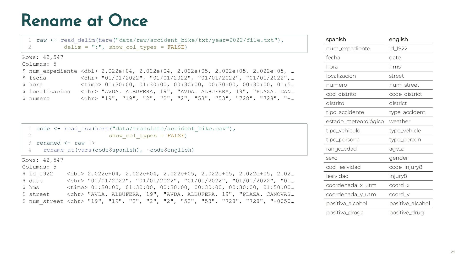
hms
    localizacion street
    numero num_street
    cod_distrito code_district
    distrito district
    tipo_accidente type_accident
    estado_meteorológico weather
    tipo_vehiculo type_vehicle
    tipo_persona type_person
    rango_edad age_c
    sexo gender
    cod_lesividad code_injury8
    lesividad injury8
    coordenada_x_utm coord_x
    coordenada_y_utm coord_y
    positiva_alcohol positive_alcohol
    positiva_droga positive_drug
    raw 1
    delim = ";", show_col_types = FALSE)
    2
    Rows: 42,547
    Columns: 5
    $ num_expediente 2.022e+04, 2.022e+04, 2.022e+05, 2.022e+05, 2.022e+05, …
    $ fecha "01/01/2022", "01/01/2022", "01/01/2022", "01/01/2022",…
    $ hora 01:30:00, 01:30:00, 00:30:00, 00:30:00, 00:30:00, 01:5…
    $ localizacion "AVDA. ALBUFERA, 19", "AVDA. ALBUFERA, 19", "PLAZA. CAN…
    $ numero "19", "19", "2", "2", "2", "53", "53", "728", "728", "+…
    code 1
    show_col_types = FALSE)
    2
    renamed
    3
    rename_at(vars(code$spanish), ~code$english)
    4
    Rows: 42,547
    Columns: 5
    $ id_1922 2.022e+04, 2.022e+04, 2.022e+05, 2.022e+05, 2.022e+05, 2.02…
    $ date "01/01/2022", "01/01/2022", "01/01/2022", "01/01/2022", "01…
    $ hms 01:30:00, 01:30:00, 00:30:00, 00:30:00, 00:30:00, 01:50:00…
    $ street "AVDA. ALBUFERA, 19", "AVDA. ALBUFERA, 19", "PLAZA. CANOVAS…
    $ num_street "19", "19", "2", "2", "2", "53", "53", "728", "728", "+0050…
    21

    View Slide

  20. Type: Date & Time
    lubridate provides strong date-parsering functions.
    lubridate::ymd("2021/08/31")
    1
    [1] "2021-08-31"
    lubridate::mdy("Sep. 10, 19")
    1
    [1] "2019-09-10"
    lubridate::dmy_hm("02/04/1999 16:00", tz="America/New_York")
    1
    [1] "1999-04-02 16:00:00 EST"
    22

    View Slide

  21. renamed |> select(date, hms) |> head()
    1
    # A tibble: 6 × 2
    date hms

    1 01/01/2022 01:30
    2 01/01/2022 01:30
    3 01/01/2022 00:30
    4 01/01/2022 00:30
    5 01/01/2022 00:30
    6 01/01/2022 01:50
    renamed |>
    1
    mutate(time = lubridate::dmy_hms(str_c(date, hms), tz = "Europe/Madrid")) |>
    2
    select(date, hms, time) |>
    3
    head()
    4
    # A tibble: 6 × 3
    date hms time

    1 01/01/2022 01:30 2022-01-01 01:30:00
    2 01/01/2022 01:30 2022-01-01 01:30:00
    3 01/01/2022 00:30 2022-01-01 00:30:00
    4 01/01/2022 00:30 2022-01-01 00:30:00
    5 01/01/2022 00:30 2022-01-01 00:30:00
    6 01/01/2022 01:50 2022-01-01 01:50:00
    23

    View Slide

  22. Type: Categorical Variables
    renamed |>
    1
    mutate(
    2
    type_person = recode_factor(type_person,
    3
    "Conductor" = "Driver",
    4
    "Pasajero" = "Passenger",
    5
    "Peatón" = "Pedestrian",
    6
    "NULL"= NULL)) |>
    7
    janitor::tabyl(type_person)
    8
    type_person n percent
    Driver 34567 0.81244271
    Passenger 6503 0.15284274
    Pedestrian 1477 0.03471455
    recode_factor() finishes:
    1. Define as factor variables
    2. Order factor variable
    3. Rename & Translate (labels in plots &
    tables)
    4. Handle NA values (next slide)
    24

    View Slide

  23. Handle NA Values
    Some datasets include NA values as string format
    unique(renamed$weather) # "Se desconoce" is also essentially NA
    1
    [1] "Despejado" "NULL" "Se desconoce" "Lluvia débil"
    [5] "Nublado" "LLuvia intensa" "Granizando" "Nevando"
    Solution 1: Define NA values when you load
    sol1 1
    delim = ";", show_col_types = FALSE,
    2
    na = c("", "NA", "NULL", "Se desconoce", "Desconocido")) |>
    3
    rename(weather = "estado_meteorológico")
    4
    5
    unique(sol1$weather)
    6
    [1] "Despejado" NA "Lluvia débil" "Nublado"
    [5] "LLuvia intensa" "Granizando" "Nevando"
    Cannot use when specific numbers as NA values (9, 99,…)
    25

    View Slide

  24. Solution2: na_if()
    Works for any case. But need to write for each NA value.
    renamed |>
    1
    mutate(
    2
    weather_old = weather,# Presentation Purpose
    3
    weather = na_if(weather, "Se desconoce"),
    4
    weather = na_if(weather, "NULL"),
    5
    ) |>
    6
    select(weather_old, weather) |>
    7
    head()
    8
    # A tibble: 6 × 2
    weather_old weather

    1 Despejado Despejado
    2 Despejado Despejado
    3 NULL
    4 NULL
    5 NULL
    6 Despejado Despejado
    26

    View Slide

  25. Soltion 3: Recode as NULL
    renamed |>
    1
    mutate(
    2
    weather_spanish = weather,# Presentation Purpose
    3
    weather = recode_factor(weather,
    4
    "Despejado" = "sunny",
    5
    "Nublado" = "cloud",
    6
    "Lluvia débil" = "soft rain",
    7
    "Lluvia intensa" = "hard rain",
    8
    "LLuvia intensa" = "hard rain",
    9
    "Nevando" = "snow",
    10
    "Granizando" = "hail",
    11
    "Se desconoce" = NULL,
    12
    "NULL" = NULL)) |>
    13
    select(weather_spanish, weather) |>
    14
    head()
    15
    # A tibble: 6 × 2
    weather_spanish weather

    1 Despejado sunny
    2 Despejado sunny
    3 NULL
    4 NULL
    5 NULL
    6 Despejado sunny
    Only works for categorical variables. But practically useful.
    27

    View Slide

  26. Parquet Format
    Speed Size Keep Type Multi-Language
    csv, tsv ❌ ❌ ❌ All
    rds, RData ❌ ✔️ ✔️ ❌
    parquet ✔️ ✔️ ✔️ Python, Julia, MATLAB, Stata,...
    You can find a benchmark in Kastrun ( )
    2022
    28

    View Slide

  27. arrow::read_parquet()
    You can load parquet data as column-information only
    df 1
    here("data/cleaned/accident_bike.parquet"),
    2
    as_data_frame = TRUE)
    3
    4
    df
    5
    # A tibble: 168,574 × 23
    id_1922 date hms street num_s…¹ code_…² distr…³
    type_…⁴ weather type_…⁵


    1 2018S0178… 04/0… 9:10… CALL.… 1 1 Centro
    Colisi… sunny Motoci…
    2 2018S0178… 04/0… 9:10… CALL.… 1 1 Centro
    Colisi… sunny Turismo
    3 2019S0000… 01/0… 3:45… PASEO… 168 11 Caraba…
    Alcance Furgon…
    4 2019S0000… 01/0… 3:45… PASEO… 168 11 Caraba…
    Alcance Turismo
    5 2019S0000… 01/0… 3:45… PASEO… 168 11 Caraba…
    Alcance Turismo
    6 2019S0000 01/0 3:45 PASEO 168 11 Caraba
    info 1
    here("data/cleaned/accident_bike.parquet"),
    2
    as_data_frame = FALSE)
    3
    4
    info
    5
    Table
    168574 rows x 23 columns
    $id_1922
    $date
    $hms
    $street
    $num_street
    $code_district
    $district
    $type_accident
    $weather >
    $type_vehicle
    $type_person >
    $age_c >
    $gender >
    $code injury8
    29

    View Slide

  28. Release Parquet on Memory
    dplyr::collect() releases the loaded parquet data on memory
    You can load them after select() or filter()
    Also, group_by() and summarize() are available
    Quite useful for large datasets
    info |>
    1
    collect()
    2
    # A tibble: 168,574 × 23
    id_1922 date hms street num_s…¹ code_…² distr…³
    type_…⁴ weather type_…⁵


    1 2018S0178… 04/0… 9:10… CALL.… 1 1 Centro
    Colisi… sunny Motoci…
    2 2018S0178… 04/0… 9:10… CALL.… 1 1 Centro
    Colisi… sunny Turismo
    3 2019S0000… 01/0… 3:45… PASEO… 168 11 Caraba…
    Alcance Furgon…
    4 2019S0000… 01/0… 3:45… PASEO… 168 11 Caraba…
    Alcance Turismo
    5 2019S0000… 01/0… 3:45… PASEO… 168 11 Caraba…
    Alcance Turismo
    6 2019S0000 01/0 3:45 PASEO 168 11 Caraba
    info |>
    1
    filter(is_hospitalized) |>
    2
    select(time, gender, age_c, positive_alcohol) |>
    3
    collect()
    4
    # A tibble: 8,724 × 4
    time gender age_c positive_alcohol

    1 2019-01-01 03:50:00 Men 21-24 FALSE
    2 2019-01-01 08:05:00 Women 60-64 FALSE
    3 2019-01-01 22:15:00 Men 35-39 FALSE
    4 2019-01-01 12:29:00 Men 55-59 FALSE
    5 2019-01-02 15:00:00 Men 60-64 FALSE
    6 2019-01-02 15:00:00 Women 50-54 FALSE
    7 2019-01-02 20:45:00 Men 70-74 FALSE
    8 2019-01-03 00:42:00 Men 35-39 FALSE
    9 2019-01-03 10:30:00 Men 15-17 FALSE
    10 2019-01-03 13:25:00 Men 30-34 FALSE
    # … with 8,714 more rows
    30

    View Slide

  29. Parquet with Partitioned Dataset
    Given this structure, arrow::open_dataset() loads them as one parquet file
    A Partitioning variable (year) becomes a new variable
    For more instructions, you can refer to Mock ( )
    data/raw/accident_bike/parquet/
    1
    ├── year=2019
    2
    │ └── part-0.parquet
    3
    ├── year=2020
    4
    │ └── part-0.parquet
    5
    ├── year=2021
    6
    │ └── part-0.parquet
    7
    └── year=2022
    8
    └── part-0.parquet
    9
    info 1
    here("data/raw/accident_bike/parquet"))
    2
    info
    3
    FileSystemDataset with 4 Parquet files
    num_expediente: string
    fecha: string
    hora: string
    localizacion: string
    numero: string
    cod_distrito: int32
    distrito: string
    tipo_accidente: string
    estado_meteorológico: string
    tipo_vehiculo: string
    tipo_persona: string
    rango_edad: string
    sexo: string
    cod_lesividad: string
    lesividad: string
    2022
    31

    View Slide

  30. Cleaning Workflow
    1. Naming
    Put informative and non-misleading names
    If necessary, translate the variable names
    You can use a correspondence table and rename variables at once
    2. Determine Types
    Date: lubridate parsing functions
    Categorical: recode_factor()
    NA-values: na_if() and recode_factor()
    3. Export
    Parquet format is better than any other data format
    Parquet makes it easy to handle large datasets
    32

    View Slide

  31. Tips in Plots
    34

    View Slide

  32. Data-ink Ratio
    Maximize the data-ink ratio in a plot:
    Data-ink Ratio Principle ( )
    Tufte 2001
    Data-ink ratio :=
    Data-ink
    Total ink used to print in the graphic
    Omit all the proportions of a graphic that can be erased without losing information
    Collolary
    35

    View Slide

  33. Maximize Data-ink Ratio
    accident_bike |>
    1
    ggplot(aes(x = type_person, fill = gender)) +
    2
    geom_bar(position = "dodge")
    3
    36

    View Slide

  34. Maximize Data-ink Ratio
    Omit axis label. The title of the plot can tell them
    Omit legend label. The label “gender” does not add any information
    Omit background grids
    accident_bike |>
    1
    ggplot(aes(x = type_person, fill = gender)) +
    2
    geom_bar(position = "dodge") +
    3
    labs(x = NULL, y = NULL, fill = NULL) +
    4
    theme_minimal() +
    5
    theme(panel.grid.minor = element_blank(),
    6
    panel.grid.major.x = element_blank())
    7
    Number of Persons Hospitalized
    37

    View Slide

  35. More Readability: Order Bar Plot
    Coord flipped. Reorder the factor variables
    Put legends inside the plot to make the plot bigger
    accident_bike |>
    1
    ggplot(aes(x = fct_rev(type_person),
    2
    fill = fct_rev(gender))) +
    3
    geom_bar(position = "dodge") +
    4
    coord_flip() +
    5
    labs(x = NULL, y = NULL, fill = NULL) +
    6
    theme_minimal() +
    7
    theme(panel.grid.minor = element_blank(),
    8
    panel.grid.major.y = element_blank(),
    9
    legend.position = c(0.9, 0.1)) +
    10
    guides(fill = guide_legend(reverse = TRUE))
    11
    Number of Persons Hospitalized
    38

    View Slide

  36. More Readability: Increase Font Size
    accident_bike |>
    1
    ggplot(aes(x = fct_rev(type_person),
    2
    fill = fct_rev(gender))) +
    3
    geom_bar(position = "dodge") +
    4
    coord_flip() +
    5
    labs(x = NULL, y = NULL, fill = NULL) +
    6
    theme_minimal() +
    7
    theme(panel.grid.minor = element_blank(),
    8
    panel.grid.major.y = element_blank(),
    9
    legend.position = c(0.9, 0.1),
    10
    axis.text.x = element_text(size = 20),
    11
    axis.text.y = element_text(size = 25),
    12
    legend.text = element_text(size = 20)) +
    13
    guides(fill = guide_legend(reverse = TRUE))
    14
    Number of Persons Hospitalized
    39

    View Slide

  37. R Color Brewer’s Palettes
    40

    View Slide

  38. R Color Brewer’s Palettes
    accident_bike |>
    1
    ggplot(aes(x = fct_rev(type_person),
    2
    fill = fct_rev(gender))) +
    3
    geom_bar(position = "dodge") +
    4
    coord_flip() +
    5
    labs(x = NULL, y = NULL, fill = NULL) +
    6
    scale_fill_brewer(palette = "Accent") +
    7
    theme_minimal() +
    8
    theme(panel.grid.minor = element_blank(),
    9
    panel.grid.major.y = element_blank(),
    10
    legend.position = c(0.9, 0.1),
    11
    axis.text.x = element_text(size = 20),
    12
    axis.text.y = element_text(size = 25),
    13
    legend.text = element_text(size = 20)) +
    14
    guides(fill = guide_legend(reverse = TRUE))
    15
    Number of Persons Hospitalized
    41

    View Slide

  39. Color-Safe Pallette: Okabe-Ito Palette
    accident_bike |>
    1
    ggplot(aes(x = fct_rev(type_person),
    2
    fill = fct_rev(gender))) +
    3
    geom_bar(position = "dodge") +
    4
    coord_flip() +
    5
    labs(x = NULL, y = NULL, fill = NULL) +
    6
    see::scale_fill_okabeito() +
    7
    theme_minimal() +
    8
    theme(panel.grid.minor = element_blank(),
    9
    panel.grid.major.y = element_blank(),
    10
    legend.position = c(0.9, 0.1),
    11
    axis.text.x = element_text(size = 20),
    12
    axis.text.y = element_text(size = 25),
    13
    legend.text = element_text(size = 20)) +
    14
    guides(fill = guide_legend(reverse = TRUE))
    15
    Number of Persons Hospitalized
    42

    View Slide

  40. Custom Palette
    accident_bike |>
    1
    ggplot(aes(x = fct_rev(type_person),
    2
    fill = fct_rev(gender))) +
    3
    geom_bar(position = "dodge") +
    4
    coord_flip() +
    5
    labs(x = NULL, y = NULL, fill = NULL) +
    6
    scale_fill_manual(values = c("#E7B800", "#00AFBB")) +
    7
    theme_minimal() +
    8
    theme(panel.grid.minor = element_blank(),
    9
    panel.grid.major.y = element_blank(),
    10
    legend.position = c(0.9, 0.1),
    11
    axis.text.x = element_text(size = 20),
    12
    axis.text.y = element_text(size = 25),
    13
    legend.text = element_text(size = 20)) +
    14
    guides(fill = guide_legend(reverse = TRUE))
    15
    Number of Persons Hospitalized
    43

    View Slide

  41. Fonts
    You can download well-designed free fonts
    My recommendation: Condensed fonts
    Roboto Condensed, Fira Sans Condensed, IBM Plex Sans
    Condensed,…
    Goolge Fonts
    Your collaborators need to download the
    fonts
    font_add_google() and showtext_auto()
    automatically solve the problem
    showtext
    44

    View Slide

  42. Roboto Condensed
    library(showtext)
    1
    font_base 2
    font_light 3
    font_add_google(font_base, font_light)
    4
    showtext_auto()
    5
    6
    accident_bike |>
    7
    ggplot(aes(x = fct_rev(type_person), fill = fct_rev(g
    8
    geom_bar(position = "dodge") +
    9
    coord_flip() +
    10
    labs(x = NULL, y = NULL, fill = NULL) +
    11
    see::scale_fill_okabeito() +
    12
    theme_minimal() +
    13
    theme(panel.grid.minor = element_blank(),
    14
    panel.grid.major.y = element_blank(),
    15
    legend.position = c(0.9, 0.1),
    16
    axis.text.x = element_text(size = 20, family =
    17
    axis.text.y = element_text(size = 25, family =
    18
    legend text = element text(size = 20 family =
    19
    Number of Persons Hospitalized
    45

    View Slide

  43. Global Options
    Don’t worry. You can set the default theme before plotting. (e.g. Scherer ( ))
    Alternatively, create a custom theme and color palette (e.g. Heiss ( ))
    2021
    theme_set(theme_minimal(base_size = 12, base_family = "Roboto Condensed"))
    1
    theme_update(
    2
    axis.ticks = element_line(color = "grey92"),
    3
    axis.ticks.length = unit(.5, "lines"),
    4
    panel.grid.minor = element_blank(),
    5
    legend.title = element_text(size = 12),
    6
    legend.text = element_text(color = "grey30"),
    7
    plot.title = element_text(size = 18, face = "bold"),
    8
    plot.subtitle = element_text(size = 12, color = "grey30"),
    9
    plot.caption = element_text(size = 9, margin = margin(t = 15))
    10
    )
    11
    2021
    46

    View Slide

  44. Third-party Themes: hrbrthemes
    accident_bike |>
    1
    ggplot(aes(x = fct_rev(type_person),
    2
    fill = fct_rev(gender))) +
    3
    geom_bar(position = "dodge") +
    4
    coord_flip() +
    5
    labs(x = NULL, y = NULL, fill = NULL) +
    6
    hrbrthemes::scale_fill_ipsum() +
    7
    hrbrthemes::theme_ipsum_rc() +
    8
    theme(panel.grid.minor = element_blank(),
    9
    panel.grid.major.y = element_blank(),
    10
    legend.position = c(0.9, 0.1),
    11
    axis.text.x = element_text(size = 20),
    12
    axis.text.y = element_text(size = 25),
    13
    legend.text = element_text(size = 20)) +
    14
    guides(fill = guide_legend(reverse = TRUE))
    15
    Number of Persons Hospitalized
    47

    View Slide

  45. Third-party Themes:: ggpubr & ggsci Plaette
    p
    1
    ggplot(aes(x = fct_rev(type_person),
    2
    fill = fct_rev(gender))) +
    3
    geom_bar(position = "dodge") +
    4
    coord_flip() +
    5
    labs(x = NULL, y = NULL, fill = NULL) +
    6
    ggpubr::theme_pubr() +
    7
    theme(panel.grid.minor = element_blank(),
    8
    panel.grid.major.y = element_blank(),
    9
    legend.position = c(0.9, 0.1),
    10
    axis.text.x = element_text(size = 20),
    11
    axis.text.y = element_text(size = 25),
    12
    legend.text = element_text(size = 20)) +
    13
    guides(fill = guide_legend(reverse = TRUE))
    14
    15
    ggpubr::set_palette(p, "jco") # choose one of ggsci pal
    16
    Number of Persons Hospitalized
    48

    View Slide

  46. Patchwork
    library(patchwork)
    1
    2
    (p_default + p_custom) / (p_hrbrthemes + p_ggpubr)
    3
    49

    View Slide

  47. Takeaway
    Maximize Data-ink Ratio
    Omit all the unnecessary elements in a plot
    Colors & Fonts
    Color Palette: RColorBrewer, Okabe-Ito, ggsci
    Fonts: Google Fonts with showtext. Especially, condensed fonts.
    Ready-made Themes: hrbrthemes, ggpubr
    Further Readings (Online Books)
    “Data Visualization: A Practical Introduction” Healy ( )
    “Fundamentals of Data Visualization” Wilke ( )
    2018
    2019
    50

    View Slide

  48. Automated Table Creation
    52

    View Slide

  49. kableExtra: Example
    tab
    1
    # A tibble: 6 × 9
    # Groups: weather [6]
    weather n_Men_2019 n_Men_2…¹ n_Men…² n_Men…³ n_Wom…⁴ n_Wom…⁵
    n_Wom…⁶ n_Wom…⁷


    1 sunny 24399 14969 19208 19420 11971 6958
    9417 9298
    2 cloud 1159 1190 1325 1633 555 554
    630 774
    3 soft rain 2126 1198 1281 1408 1068 542
    605 716
    4 hard rain 386 202 386 352 222 96
    210 179
    5 snow 2 2 124 5 NA NA
    38 1
    library(kableExtra)
    1
    options(knitr.kable.NA = '')
    2
    3
    ktb
    4
    kbl(format = "latex", booktabs = TRUE,
    5
    col.names = c(" ", 2019:2022, 2019:2022)) |>
    6
    add_header_above(c(" ", "Men" = 4, "Women" = 4)) |>
    7
    pack_rows(index = c("Good" = 2, "Bad" = 4))
    8
    9
    ktb |>
    10
    save_kable(here("output/tex/kableextra/tb_accident_bike.tex"))
    11
    booktabs = TRUE for booktabs
    package in LaTeX
    You can specify the column names
    by col.names
    You can pack columns and rows by
    add_header_above() and
    pack_rows()
    save_kable() saves in a tex file if the
    file name ends with “.tex”
    53

    View Slide

  50. kableExtra
    Dataframe (tibble) to Table
    Create a tibble table by dplyr::group_by & dpyr::summarize and
    janitor::tabyl()
    For regression tables, you can use modelsummary (next slide)
    Pack Columns and Rows
    As far as I know, Python, Julia, and Stata do not allow us to pack them easily
    More Complicated Tables
    You can refer to Hao Zhu’s
    If a table contains a mathematical expression, use escape=FALSE. See a
    discussion in
    document
    stacoverflow
    54

    View Slide

  51. modelsummary
    Given the following regression results,
    library(fixest) # for faster regression with fixed effect
    1
    2
    models 3
    "(1)" = feglm(is_hospitalized ~ type_person + positive_alcohol + positive_drug | age_c + gender,
    4
    family = binomial(logit), data = data),
    5
    "(2)" = feglm(is_hospitalized ~ type_person + positive_alcohol + positive_drug | age_c + gender + type_vehicle,
    6
    family = binomial(logit), data = data),
    7
    "(3)" = feglm(is_hospitalized ~ type_person + positive_alcohol + positive_drug | age_c + gender + type_vehicle +
    8
    family = binomial(logit), data = data),
    9
    "(4)" = feglm(is_died ~ type_person + positive_alcohol + positive_drug | age_c + gender,
    10
    family = binomial(logit), data = data),
    11
    "(5)" = feglm(is_died ~ type_person + positive_alcohol + positive_drug | age_c + gender + type_vehicle,
    12
    family = binomial(logit), data = data),
    13
    "(6)" = feglm(is_died ~ type_person + positive_alcohol + positive_drug | age_c + gender + type_vehicle + weather,
    14
    family = binomial(logit), data = data)
    15
    )
    16
    55

    View Slide

  52. modelsummary: Init
    (1) (2) (3) (4) (5) (6)
    type_personPassenger 0.049 0.530 0.507 −1.781 −1.575 −1.565
    (0.104) (0.071) (0.070) (0.759) (0.783) (0.784)
    type_personPedestrian 2.124 2.402 2.323 2.280 2.418 2.422
    (0.115) (0.066) (0.064) (0.301) (0.287) (0.285)
    positive_alcoholTRUE −0.077 0.310 0.353 −13.710 −13.455 −13.492
    (0.088) (0.095) (0.093) (0.053) (0.064) (0.063)
    Num.Obs. 149918 149831 134006 90852 89300 86330
    R2 0.055 0.171 0.165 0.107 0.145 0.148
    R2 Adj. 0.054 0.170 0.163 0.086 0.113 0.112
    R2 Within 0.047 0.054 0.052 0.073 0.076 0.076
    R2 Within Adj. 0.047 0.054 0.052 0.070 0.072 0.073
    AIC 62871.0 55210.6 53565.4 1601.9 1552.2 1534.5
    BIC 63079.3 55696.5 54085.1 1780.8 1824.8 1834.2
    RMSE 0.23 0.22 0.23 0.04 0.04 0.04
    Std.Errors by: age_c by: age_c by: age_c by: age_c by: age_c by: age_c
    FE: age_c X X X X X X
    FE: gender X X X X X X
    FE: type_vehicle X X X X
    FE: weather X X
    modelsummary(models)
    1
    56

    View Slide

  53. modelsummary: Modify Coefficients
    (1) (2) (3) (4) (5) (6)
    Passenger 0.049 0.530 0.507 −1.781 −1.575 −1.565
    (0.104) (0.071) (0.070) (0.759) (0.783) (0.784)
    Pedestrian 2.124 2.402 2.323 2.280 2.418 2.422
    (0.115) (0.066) (0.064) (0.301) (0.287) (0.285)
    Positive Alcohol −0.077 0.310 0.353 −13.710 −13.455 −13.492
    (0.088) (0.095) (0.093) (0.053) (0.064) (0.063)
    Num.Obs. 149918 149831 134006 90852 89300 86330
    R2 0.055 0.171 0.165 0.107 0.145 0.148
    R2 Adj. 0.054 0.170 0.163 0.086 0.113 0.112
    R2 Within 0.047 0.054 0.052 0.073 0.076 0.076
    R2 Within Adj. 0.047 0.054 0.052 0.070 0.072 0.073
    AIC 62871.0 55210.6 53565.4 1601.9 1552.2 1534.5
    BIC 63079.3 55696.5 54085.1 1780.8 1824.8 1834.2
    RMSE 0.23 0.22 0.23 0.04 0.04 0.04
    Std.Errors by: age_c by: age_c by: age_c by: age_c by: age_c by: age_c
    FE: age_c X X X X X X
    FE: gender X X X X X X
    FE: type_vehicle X X X X
    FE: weather X X
    cm 1
    "type_personPassenger" = "Passenger",
    2
    "type_personPedestrian" = "Pedestrian",
    3
    "positive_alcoholTRUE" = "Positive Alcohol"
    4
    )
    5
    6
    modelsummary(models,
    7
    coef_map = cm
    8
    )
    9
    57

    View Slide

  54. modelsummary: Modify Statitics
    (1) (2) (3) (4) (5) (6)
    Passenger 0.049 0.530 0.507 −1.781 −1.575 −1.565
    (0.104) (0.071) (0.070) (0.759) (0.783) (0.784)
    Pedestrian 2.124 2.402 2.323 2.280 2.418 2.422
    (0.115) (0.066) (0.064) (0.301) (0.287) (0.285)
    Positive Alcohol −0.077 0.310 0.353 −13.710 −13.455 −13.492
    (0.088) (0.095) (0.093) (0.053) (0.064) (0.063)
    Observations 149918 149831 134006 90852 89300 86330
    FE: Age Group X X X X X X
    FE: Gender X X X X X X
    FE: Type of Vehicle X X X X
    FE: Weather X X
    cm 1
    "type_personPassenger" = "Passenger",
    2
    "type_personPedestrian" = "Pedestrian",
    3
    "positive_alcoholTRUE" = "Positive Alcohol"
    4
    )
    5
    6
    gm 7
    raw = c("nobs", "FE: age_c", "FE: gender", "FE: type_vehicle",
    8
    clean = c("Observations", "FE: Age Group", "FE: Gender", "FE: T
    9
    fmt = c(0, 0, 0, 0, 0)
    10
    )
    11
    12
    modelsummary(models,
    13
    coef_map = cm,
    14
    gof_map = gm
    15
    )
    16
    58

    View Slide

  55. modelsummary: Stars & Headers
    Hospitalization Died within 24 hours
    (1) (2) (3) (4) (5) (6)
    Passenger 0.049 0.530** 0.507** −1.781* −1.575+ −1.565+
    (0.104) (0.071) (0.070) (0.759) (0.783) (0.784)
    Pedestrian 2.124** 2.402** 2.323** 2.280** 2.418** 2.422**
    (0.115) (0.066) (0.064) (0.301) (0.287) (0.285)
    Positive Alcohol −0.077 0.310** 0.353** −13.710** −13.455** −13.492**
    (0.088) (0.095) (0.093) (0.053) (0.064) (0.063)
    Observations 149918 149831 134006 90852 89300 86330
    FE: Age Group X X X X X X
    FE: Gender X X X X X X
    FE: Type of Vehicle X X X X
    FE: Weather X X
    + p < 0.1, * p < 0.05, ** p < 0.01
    code-line-numbers="7,16"
    1
    cm 2
    "type_personPassenger" = "Passenger",
    3
    "type_personPedestrian" = "Pedestrian",
    4
    "positive_alcoholTRUE" = "Positive Alcohol"
    5
    )
    6
    7
    gm 8
    raw = c("nobs", "FE: age_c", "FE: gender", "FE: type_vehicle",
    9
    clean = c("Observations", "FE: Age Group", "FE: Gender", "FE: T
    10
    fmt = c(0, 0, 0, 0, 0)
    11
    )
    12
    13
    modelsummary(models,
    14
    stars = c("+" = .1, "*" = .05, "**" = .01),
    15
    coef_map = cm,
    16
    gof_map = gm) |>
    17
    add_header_above(c(" ", "Hospitalization" = 3, "Died within 24 ho
    18
    59

    View Slide

  56. modelsummary: Export to
    output = "latex_tabular" produces a tex file not containing table tag
    LT X
    A
    E
    cm 1
    "type_personPassenger" = "Passenger",
    2
    "type_personPedestrian" = "Pedestrian",
    3
    "positive_alcoholTRUE" = "Positive Alcohol"
    4
    )
    5
    6
    gm 7
    raw = c("nobs", "FE: age_c", "FE: gender", "FE: type_vehicle",
    8
    clean = c("Observations", "FE: Age Group", "FE: Gender", "FE: T
    9
    fmt = c(0, 0, 0, 0, 0)
    10
    )
    11
    12
    modelsummary(models,
    13
    output = "latex_tabular",
    14
    stars = c("+" = .1, "*" = .05, "**" = .01),
    15
    coef_map = cm,
    16
    gof_map = gm) |>
    17
    add_header_above(c(" ", "Hospitalization" = 3, "Died within 24 ho
    18
    row spec(7 hline after = T) |>
    19
    60

    View Slide

  57. Takeaway
    kableExtra & modelsummary
    You can quickly export tibble (dataframe) as latex table by kableExtra
    modelsummary produces kableExtra object from regression results
    You can see the latex table in output/tex/ and the compiled results in
    code/thesis/
    Further Readings
    Official Document and Zhu ( )
    is a great alternative to kableExtra. I use gt tables in my slides
    modelsummary 2021
    gt
    61

    View Slide

  58. Quarto
    63

    View Slide

  59. What Is Quarto (.qmd)?
    knitr
    jupyter
    pandoc
    qmd md
    I use Quarto for
    Reporting: Easy to show the progress to supervisor/coauthors
    Presentation: Reveal.js produces reasonably beautiful slides
    64

    View Slide

  60. Quarto (Markdown) Is Easy-version of !
    Quarto (Markdown)
    Headings
    Bullet points
    Enumerate
    LT X
    A
    E
    # Heading 1
    1
    ## Heading 2
    2
    ### Heading 3
    3
    LT X
    A
    E
    \section{Heading 1}
    1
    \subsection{Heading 2}
    2
    \subsubsection{Heading 3}
    3
    - item 1
    1
    - item 2
    2
    - item 3
    3
    \begin{itemize}
    1
    \item item 1
    2
    \item item 2
    3
    \item item 3
    4
    \end{itemize}
    5
    1. item 1
    1
    1. item 2
    2
    1. item 3
    3
    \begin{enumerate}
    1
    \item item 1
    2
    \item item 2
    3
    \item item 3
    4
    \end{enumerate}
    5
    65

    View Slide

  61. Quarto (Markdown) Is Easy-version of !
    Quarto (Markdown)
    Text Formatting
    Display Math
    Cross References
    LT X
    A
    E
    **bold letters**
    1
    _italic letters_
    2
    $f_n(x)$
    3
    LT X
    A
    E
    \textbf{bold letters}
    1
    \textit{italic letters}
    2
    $f_n(x)$
    3
    $$
    1
    \begin{aligned}
    2
    u(x) &= \frac{c^{1 - \gamma}}{1 - \gamma} \\
    3
    u'(x) &= c^{1- \gamma}
    4
    \end{aligned}
    5
    $$
    6
    \begin{align*}
    1
    u(x) &= \frac{c^{1 - \gamma}}{1 - \gamma} \\
    2
    u'(x) &= c^{1- \gamma}
    3
    \end{align*}
    4
    @bib_tex_key
    1
    @fig-label_fig
    2
    @tbl-label_tbl
    3
    \cite(bib_tex_key)
    1
    \ref{fig:label_fig}
    2
    \ref{tbl:label_tbl}
    3
    66

    View Slide

  62. Quarto Presentation
    Quarto (Reveal.js) (Beamer)
    ## First Slide
    1
    2
    Blah, Blah, Blah
    3
    4
    ## Second Slide
    5
    6
    Yeah, Yeah, Yeah
    7
    LT X
    A
    E
    \begin{frame}{First Slide}
    1
    2
    Blah, Blah, Blah
    3
    4
    \end{frame}
    5
    6
    \begin{frame}{Secon Slide}
    7
    8
    Yeah, Yeah, Yeah
    9
    10
    \end{frame}
    11
    67

    View Slide

  63. Quarto Presentation: Fragments
    Quarto (Reveal.js)
    Pause
    (Beamer)
    Incremental List
    For more complicated examples, see Tom Mock’s of the slides
    First fragment
    1
    2
    . . .
    3
    4
    Second fragment
    5
    LT X
    A
    E
    First fragment
    1
    2
    \pause
    3
    4
    Second fragment
    5
    ::: {.incremental}
    1
    2
    - 1st element
    3
    - 2nd element
    4
    - 3rd element
    5
    6
    :::
    7
    \begin{itemize}[]
    1
    \item 1st element
    2
    \item 2nd element
    3
    \item 3rd element
    4
    \end{itemize}
    5
    this part
    68

    View Slide

  64. Why Do I Use Quarto?
    Reports
    Analysis, Results, and Interpretation are done in one file
    Easy to communicate with supervisor/coauthors
    Presentations
    I prefer its design to Beamer. Highly customizable
    Same effort as Beamer slides. The syntax is almost the same
    For more reasons and techniques, read my blog
    69

    View Slide

  65. References
    Boswell, Dustin, and Trevor Foucher. 2011. The Art of Readable Code. 1st ed. Theory in Practice. Sebastopol, Calif:
    O’Reilly.
    Bryan, Jenny. 2018. “Zen And The aRt Of Workflow Maintenance.” Part of 47 JAIIO.
    .
    Healy, Kieran. 2018. Data Visualization: A Practical Introduction. 1st edition. Princeton, NJ: Princeton University Press.
    .
    Heiss, Andrew. 2021. “Who Cares About Crackdowns? Exploring the Role of Trust in Individual Philanthropy.”
    .
    Kastrun, Tomaz. 2022. “Comparing Performances of CSV to RDS, Parquet, and Feather File Formats in R R-Bloggers.”
    R-bloggers. R-Bloggers.
    .
    Mock, Tom. 2022. “Outrageously Efficient Exploratory Data Analysis with Apache Arrow and Dplyr.” Voltron Data.
    .
    Scherer, C’edric. 2021. “Ggplot Wizardry: My Favorite Tricks and Secrets for Beautiful Plots in R.” Online.
    .
    Tufte, Edward R. 2001. The Visual Display of Quantitative Information. Cheshire, Conn.
    Wilke, Claus O. 2019. Fundamentals of Data Visualization: A Primer on Making Informative and Compelling
    Figures. Sebastopol, CA. .
    Zhu, Hao. 2021. “Create Awesome LaTeX Table with Knitr::kable and kableExtra,” February.
    .
    https://github.com/jennybc/zen-
    art-workflow
    https://socviz.co/
    https://github.com/andrewheiss/who-cares-about-
    crackdown/blob/ad6312957de927674a5da2437a2f993e52f53d88/R/graphics.R
    https://www.r-bloggers.com/2022/05/comparing-performances-of-csv-to-rds-parquet-
    and-feather-file-formats-in-r/
    https://jthomasmock.github.io/arrow-dplyr/
    https://www.cedricscherer.com/slides/useR-2021_ggplot-wizardry-extended.pdf
    https://clauswilke.com/dataviz/
    https://cran.r-
    project.org/web/packages/kableExtra/vignettes/awesome_table_in_pdf.pdf
    70

    View Slide