thesis An Efficient and Parallel Abstract Interpreter in Scala — Second Presentation — Olivier Pirson — [email protected] orcid.org/0000-0001-6296-9659 March 20, 2018 (Little corrections: July 1st, 2018) https://bitbucket.org/OPiMedia/efficient-parallel-abstract-interpreter-in-scala Vrije Universiteit Brussel Promotors Coen De Roover Wolfgang De Meuter Advisor Quentin Stievenart
Presentation The context: Abstract Interpretation for Static Analysis The problematic: Too heavy for real programs Parallel algorithms Done and todo References 1 The context: Abstract Interpretation for Static Analysis 2 The problematic: Too heavy for real programs 3 Parallel algorithms 4 Done and todo 5 References An Efficient and Parallel Abstract Interpreter in Scala — Second Presentation 2 / 21
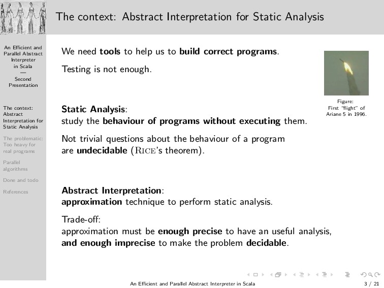
Presentation The context: Abstract Interpretation for Static Analysis The problematic: Too heavy for real programs Parallel algorithms Done and todo References The context: Abstract Interpretation for Static Analysis We need tools to help us to build correct programs. Figure: First “flight” of Ariane 5 in 1996. Testing is not enough. Static Analysis: study the behaviour of programs without executing them. Not trivial questions about the behaviour of a program are undecidable (Rice’s theorem). Abstract Interpretation: approximation technique to perform static analysis. Trade-off: approximation must be enough precise to have an useful analysis, and enough imprecise to make the problem decidable. An Efficient and Parallel Abstract Interpreter in Scala — Second Presentation 3 / 21
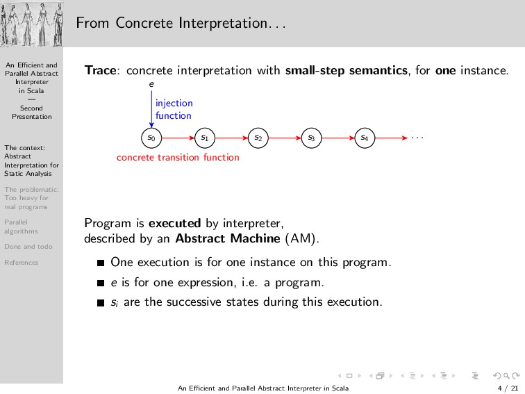
Presentation The context: Abstract Interpretation for Static Analysis The problematic: Too heavy for real programs Parallel algorithms Done and todo References From Concrete Interpretation. . . Trace: concrete interpretation with small-step semantics, for one instance. e s0 s1 s2 s3 s4 · · · injection function concrete transition function Program is executed by interpreter, described by an Abstract Machine (AM). One execution is for one instance on this program. e is for one expression, i.e. a program. si are the successive states during this execution. An Efficient and Parallel Abstract Interpreter in Scala — Second Presentation 4 / 21
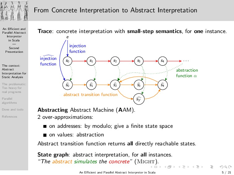
Presentation The context: Abstract Interpretation for Static Analysis The problematic: Too heavy for real programs Parallel algorithms Done and todo References From Concrete Interpretation to Abstract Interpretation Trace: concrete interpretation with small-step semantics, for one instance. e s0 s1 s2 s3 s4 · · · s0 s1 s2 s3 s4 s3′ injection function injection function abstract transition function abstraction function α Abstracting Abstract Machine (AAM). 2 over-approximations: on addresses: by modulo; give a finite state space on values: abstraction Abstract transition function returns all directly reachable states. State graph: abstract interpretation, for all instances. “The abstract simulates the concrete” (Might). An Efficient and Parallel Abstract Interpreter in Scala — Second Presentation 5 / 21
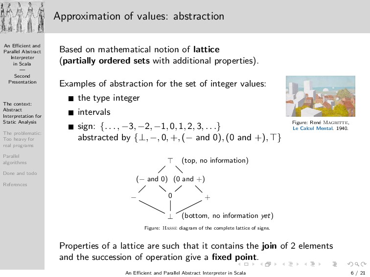
Presentation The context: Abstract Interpretation for Static Analysis The problematic: Too heavy for real programs Parallel algorithms Done and todo References Approximation of values: abstraction Based on mathematical notion of lattice (partially ordered sets with additional properties). Examples of abstraction for the set of integer values: Figure: Ren´ e Magritte, Le Calcul Mental. 1940. the type integer intervals sign: {. . . , −3, −2, −1, 0, 1, 2, 3, . . .} abstracted by {⊥, −, 0, +, (− and 0), (0 and +), ⊤} ⊤ (top, no information) (− and 0) (0 and +) − 0 + ⊥ (bottom, no information yet) Figure: Hasse diagram of the complete lattice of signs. Properties of a lattice are such that it contains the join of 2 elements and the succession of operation give a fixed point. An Efficient and Parallel Abstract Interpreter in Scala — Second Presentation 6 / 21
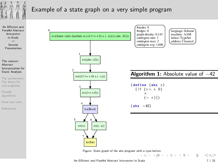
Presentation The context: Abstract Interpretation for Static Analysis The problematic: Too heavy for real programs Parallel algorithms Done and todo References Example of a state graph on a very simple program ev((letrec ((abs (lambda (x) (if (>= x 0) x (- x))))) (abs -42))) 0 ev((abs -42)) 1 ev((if (>= x 0) x (- x))) 2 ev((>= x 0)) 3 ko(Bool) 4 ev(x) 5 ev((- x)) 6 ko(Int) 7 #nodes: 8 #edges: 8 graph density: 0,143 outdegree min: 1 outdegree max: 2 outdegree avg: 1,000 language: Scheme machine: AAM lattice: TypeSet address: Classical Figure: State graph of the abs program with a type lattice. Algorithm 1: Absolute value of −42 ( Ò ( × x ) ( i f (>= x 0) x (− x ) ) ) ( × −42) An Efficient and Parallel Abstract Interpreter in Scala — Second Presentation 7 / 21
Presentation The context: Abstract Interpretation for Static Analysis The problematic: Too heavy for real programs Parallel algorithms Done and todo References 1 The context: Abstract Interpretation for Static Analysis 2 The problematic: Too heavy for real programs 3 Parallel algorithms 4 Done and todo 5 References An Efficient and Parallel Abstract Interpreter in Scala — Second Presentation 8 / 21
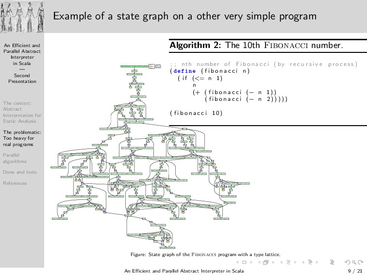
Presentation The context: Abstract Interpretation for Static Analysis The problematic: Too heavy for real programs Parallel algorithms Done and todo References Example of a state graph on a other very simple program ev((letrec ((fibonacci (lambda (n) (if (<= n 1) n (+ (fibonacci (- n 1)) (fibonacci (- n 2))))))) (fibonacci 10))) 0 ev((fibonacci 10)) 1 ev((if (<= n 1) n (+ (fibonacci (- n 1)) (fibonacci (- n 2))))) 2 ev((<= n 1)) 3 ko(Bool) 4 ev(n) 5 ev((+ (fibonacci (- n 1)) (fibonacci (- n 2)))) 6 ko(Int) 7 ev((fibonacci (- n 1))) 8 ev((- n 1)) 9 ko(Int) 10 ev((if (<= n 1) n (+ (fibonacci (- n 1)) (fibonacci (- n 2))))) 11 ev((<= n 1)) 12 ko(Bool) 13 ev(n) 14 ev((+ (fibonacci (- n 1)) (fibonacci (- n 2)))) 15 ev(n) 16 ev((+ (fibonacci (- n 1)) (fibonacci (- n 2)))) 17 ko(Int) 18 ev((fibonacci (- n 1))) 19 ko(Int) 20 ev((fibonacci (- n 1))) 21 ev((- n 1)) 22 ev((fibonacci (- n 2))) 23 ev((- n 1)) 24 ko(Int) 25 ev((- n 2)) 26 ko(Int) 27 ev((if (<= n 1) n (+ (fibonacci (- n 1)) (fibonacci (- n 2))))) 28 ko(Int) 29 ev((if (<= n 1) n (+ (fibonacci (- n 1)) (fibonacci (- n 2))))) 30 ev((if (<= n 1) n (+ (fibonacci (- n 1)) (fibonacci (- n 2))))) 31 ev((<= n 1)) 32 ev((<= n 1)) 33 ko(Bool) 34 ko(Bool) 35 ev(n) 36 ev((+ (fibonacci (- n 1)) (fibonacci (- n 2)))) 37 ev(n) 38 ev((+ (fibonacci (- n 1)) (fibonacci (- n 2)))) 39 ev((+ (fibonacci (- n 1)) (fibonacci (- n 2)))) 40 ev((+ (fibonacci (- n 1)) (fibonacci (- n 2)))) 41 ev(n) 42 ev((+ (fibonacci (- n 1)) (fibonacci (- n 2)))) 43 ev(n) 44 ev(n) 45 ko(Int) 46 ko(Int) 47 ev((fibonacci (- n 1))) 49 ev((fibonacci (- n 1))) 52 ko(Int) 48 ev((fibonacci (- n 1))) 51 ko(Int) 50 ko(Int) 53 ev((fibonacci (- n 2))) 54 ev((fibonacci (- n 2))) 55 ev((- n 1)) 56 ev((- n 1)) 57 ev((- n 1)) 58 ev((fibonacci (- n 2))) 59 ev((- n 2)) 60 ev((- n 2)) 61 ko(Int) 62 ko(Int) 63 ko(Int) 64 ev((- n 2)) 65 ko(Int) 66 ko(Int) 67 ev((if (<= n 1) n (+ (fibonacci (- n 1)) (fibonacci (- n 2))))) 68 ev((if (<= n 1) n (+ (fibonacci (- n 1)) (fibonacci (- n 2))))) 69 ev((if (<= n 1) n (+ (fibonacci (- n 1)) (fibonacci (- n 2))))) 70 ko(Int) 71 ev((if (<= n 1) n (+ (fibonacci (- n 1)) (fibonacci (- n 2))))) 72 ev((if (<= n 1) n (+ (fibonacci (- n 1)) (fibonacci (- n 2))))) 73 ev((<= n 1)) 74 ev((<= n 1)) 75 ev((if (<= n 1) n (+ (fibonacci (- n 1)) (fibonacci (- n 2))))) 76 ev((<= n 1)) 77 ko(Bool) 78 ko(Bool) 79 ko(Bool) 80 ev(n) 81 ev(n) 82 ev((+ (fibonacci (- n 1)) (fibonacci (- n 2)))) 83 ev((+ (fibonacci (- n 1)) (fibonacci (- n 2)))) 84 ev(n) 85 ev((+ (fibonacci (- n 1)) (fibonacci (- n 2)))) 86 ev(n) 87 ev((+ (fibonacci (- n 1)) (fibonacci (- n 2)))) 88 ev(n) 89 ev((+ (fibonacci (- n 1)) (fibonacci (- n 2)))) 90 ev((+ (fibonacci (- n 1)) (fibonacci (- n 2)))) 91 ev(n) 92 ev(n) 93 ev((+ (fibonacci (- n 1)) (fibonacci (- n 2)))) 94 ev((+ (fibonacci (- n 1)) (fibonacci (- n 2)))) 95 ev(n) 96 ev((+ (fibonacci (- n 1)) (fibonacci (- n 2)))) 97 ev(n) 98 ko(Int) 100 ko(Int) 99 ev((fibonacci (- n 1))) 101 ko(Int) 102 ko(Int) 103 ko(Int) 105 ko(Int) 104 ko(Int) 109 ev((fibonacci (- n 1))) 106 ev((fibonacci (- n 1))) 110 ko(Int) 108 ko(Int) 107 ev((fibonacci (- n 2))) 111 ev((fibonacci (- n 2))) 112 ev((- n 1)) 113 ev((fibonacci (- n 2))) 114 ev((fibonacci (- n 2))) 115 ev((- n 1)) 116 ev((fibonacci (- n 2))) 117 ev((- n 1)) 118 ev((- n 2)) 119 ev((- n 2)) 120 ko(Int) 121 ev((- n 2)) 122 ev((- n 2)) 123 ko(Int) 124 ev((- n 2)) 125 ko(Int) 126 ko(Int) 127 ko(Int) 128 ev((if (<= n 1) n (+ (fibonacci (- n 1)) (fibonacci (- n 2))))) 129 ko(Int) 130 ko(Int) 131 ev((if (<= n 1) n (+ (fibonacci (- n 1)) (fibonacci (- n 2))))) 132 ko(Int) 133 ev((if (<= n 1) n (+ (fibonacci (- n 1)) (fibonacci (- n 2))))) 134 ev((if (<= n 1) n (+ (fibonacci (- n 1)) (fibonacci (- n 2))))) 135 ev((if (<= n 1) n (+ (fibonacci (- n 1)) (fibonacci (- n 2))))) 136 ev((<= n 1)) 137 ev((if (<= n 1) n (+ (fibonacci (- n 1)) (fibonacci (- n 2))))) 138 ev((if (<= n 1) n (+ (fibonacci (- n 1)) (fibonacci (- n 2))))) 139 ev((if (<= n 1) n (+ (fibonacci (- n 1)) (fibonacci (- n 2))))) 140 ev((<= n 1)) 141 ev((<= n 1)) 142 ko(Bool) 143 ev((<= n 1)) 144 ko(Bool) 145 ko(Bool) 146 ev(n) 147 ev((+ (fibonacci (- n 1)) (fibonacci (- n 2)))) 148 ev((+ (fibonacci (- n 1)) (fibonacci (- n 2)))) 149 ev(n) 150 ev((+ (fibonacci (- n 1)) (fibonacci (- n 2)))) 151 ev(n) 152 ko(Bool) 153 ev((+ (fibonacci (- n 1)) (fibonacci (- n 2)))) 154 ev((+ (fibonacci (- n 1)) (fibonacci (- n 2)))) 155 ev(n) 156 ev((+ (fibonacci (- n 1)) (fibonacci (- n 2)))) 157 ev(n) 158 ev(n) 159 ev(n) 160 ev((+ (fibonacci (- n 1)) (fibonacci (- n 2)))) 161 ev((+ (fibonacci (- n 1)) (fibonacci (- n 2)))) 162 ev(n) 163 ev(n) 164 ev((+ (fibonacci (- n 1)) (fibonacci (- n 2)))) 165 ko(Int) 167 ko(Int) 168 ko(Int) 166 ev(n) 169 ev((+ (fibonacci (- n 1)) (fibonacci (- n 2)))) 170 ev(n) 171 ev(n) 172 ev((+ (fibonacci (- n 1)) (fibonacci (- n 2)))) 173 ev((+ (fibonacci (- n 1)) (fibonacci (- n 2)))) 174 ko(Int) 177 ko(Int) 175 ko(Int) 176 ko(Int) 178 ev((fibonacci (- n 1))) 180 ko(Int) 181 ko(Int) 179 ev((fibonacci (- n 1))) 182 ev((fibonacci (- n 2))) 183 ev((fibonacci (- n 2))) 184 ev((fibonacci (- n 2))) 185 ko(Int) 190 ev((fibonacci (- n 1))) 187 ko(Int) 189 ko(Int) 188 ev((fibonacci (- n 1))) 186 ev((fibonacci (- n 2))) 191 ev((fibonacci (- n 2))) 192 ev((- n 1)) 193 ev((- n 1)) 194 ev((- n 2)) 195 ev((- n 2)) 196 ev((- n 2)) 197 ev((- n 1)) 198 ev((- n 1)) 199 ev((- n 2)) 200 ev((- n 2)) 201 ko(Int) 202 ko(Int) 203 ko(Int) 204 ko(Int) 205 ko(Int) 206 ko(Int) 207 ko(Int) 208 ko(Int) 209 ko(Int) 210 ev((if (<= n 1) n (+ (fibonacci (- n 1)) (fibonacci (- n 2))))) 211 ev((if (<= n 1) n (+ (fibonacci (- n 1)) (fibonacci (- n 2))))) 212 ev((if (<= n 1) n (+ (fibonacci (- n 1)) (fibonacci (- n 2))))) 213 ev((if (<= n 1) n (+ (fibonacci (- n 1)) (fibonacci (- n 2))))) 214 ev((if (<= n 1) n (+ (fibonacci (- n 1)) (fibonacci (- n 2))))) 215 ev((if (<= n 1) n (+ (fibonacci (- n 1)) (fibonacci (- n 2))))) 216 ev((if (<= n 1) n (+ (fibonacci (- n 1)) (fibonacci (- n 2))))) 217 ev((if (<= n 1) n (+ (fibonacci (- n 1)) (fibonacci (- n 2))))) 218 ev((if (<= n 1) n (+ (fibonacci (- n 1)) (fibonacci (- n 2))))) 219 ev((<= n 1)) 220 ev((<= n 1)) 221 ev((<= n 1)) 222 ko(Bool) 223 ko(Bool) 224 ko(Bool) 225 ev((+ (fibonacci (- n 1)) (fibonacci (- n 2)))) 226 ev(n) 227 ev(n) 228 ev((+ (fibonacci (- n 1)) (fibonacci (- n 2)))) 229 ev((+ (fibonacci (- n 1)) (fibonacci (- n 2)))) 230 ev(n) 231 ev((+ (fibonacci (- n 1)) (fibonacci (- n 2)))) 232 ev(n) 233 ev(n) 234 ev((+ (fibonacci (- n 1)) (fibonacci (- n 2)))) 235 ev(n) 236 ev((+ (fibonacci (- n 1)) (fibonacci (- n 2)))) 237 ev((+ (fibonacci (- n 1)) (fibonacci (- n 2)))) 238 ev(n) 239 ev((+ (fibonacci (- n 1)) (fibonacci (- n 2)))) 240 ev((+ (fibonacci (- n 1)) (fibonacci (- n 2)))) 241 ev(n) 242 ev(n) 243 ko(Int) 246 ko(Int) 244 ko(Int) 245 ko(Int) 248 ko(Int) 249 ko(Int) 247 ev((fibonacci (- n 1))) 251 ko(Int) 253 ko(Int) 250 ko(Int) 252 ev((fibonacci (- n 2))) 254 ev((- n 1)) 255 ev((- n 2)) 256 ko(Int) 257 ko(Int) 258 ev((if (<= n 1) n (+ (fibonacci (- n 1)) (fibonacci (- n 2))))) 259 ev((if (<= n 1) n (+ (fibonacci (- n 1)) (fibonacci (- n 2))))) 260 ev((<= n 1)) 261 ko(Bool) 262 ev(n) 263 ev(n) 264 ev((+ (fibonacci (- n 1)) (fibonacci (- n 2)))) 265 ev((+ (fibonacci (- n 1)) (fibonacci (- n 2)))) 266 ev(n) 267 ev((+ (fibonacci (- n 1)) (fibonacci (- n 2)))) 268 ko(Int) 271 ko(Int) 269 ev((fibonacci (- n 1))) 270 ko(Int) 272 ev((- n 1)) 273 ko(Int) 274 ev((if (<= n 1) n (+ (fibonacci (- n 1)) (fibonacci (- n 2))))) 275 #nodes: 276 #edges: 346 graph density: 0,005 outdegree min: 1 outdegree max: 6 outdegree avg: 1,254 language: Scheme machine: AAM lattice: TypeSet address: Classical Figure: State graph of the Fibonacci program with a type lattice. Algorithm 2: The 10th Fibonacci number. ; ; nth number of F i b o n a c c i ( by r e c u r s i v e p r o c e s s ) ( Ò ( f i b o n a c c i n ) ( i f (<= n 1) n (+ ( f i b o n a c c i (− n 1)) ( f i b o n a c c i (− n 2 ) ) ) ) ) ( f i b o n a c c i 10) An Efficient and Parallel Abstract Interpreter in Scala — Second Presentation 9 / 21
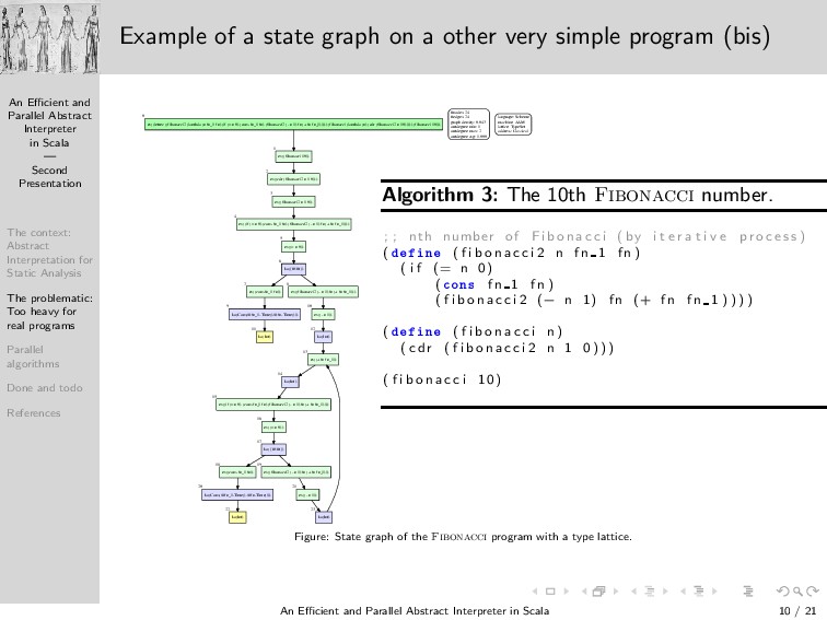
Presentation The context: Abstract Interpretation for Static Analysis The problematic: Too heavy for real programs Parallel algorithms Done and todo References Example of a state graph on a other very simple program (bis) ev((letrec ((fibonacci2 (lambda (n fn_1 fn) (if (= n 0) (cons fn_1 fn) (fibonacci2 (- n 1) fn (+ fn fn_1))))) (fibonacci (lambda (n) (cdr (fibonacci2 n 1 0))))) (fibonacci 10))) 0 ev((fibonacci 10)) 1 ev((cdr (fibonacci2 n 1 0))) 2 ev((fibonacci2 n 1 0)) 3 ev((if (= n 0) (cons fn_1 fn) (fibonacci2 (- n 1) fn (+ fn fn_1)))) 4 ev((= n 0)) 5 ko({#f,#t}) 6 ev((cons fn_1 fn)) 7 ev((fibonacci2 (- n 1) fn (+ fn fn_1))) 8 ko(Cons(@fn_1-Time(),@fn-Time())) 9 ev((- n 1)) 10 ko(Int) 11 ko(Int) 12 ev((+ fn fn_1)) 13 ko(Int) 14 ev((if (= n 0) (cons fn_1 fn) (fibonacci2 (- n 1) fn (+ fn fn_1)))) 15 ev((= n 0)) 16 ko({#f,#t}) 17 ev((cons fn_1 fn)) 18 ev((fibonacci2 (- n 1) fn (+ fn fn_1))) 19 ko(Cons(@fn_1-Time(),@fn-Time())) 20 ev((- n 1)) 21 ko(Int) 22 ko(Int) 23 #nodes: 24 #edges: 24 graph density: 0,043 outdegree min: 1 outdegree max: 2 outdegree avg: 1,000 language: Scheme machine: AAM lattice: TypeSet address: Classical Figure: State graph of the Fibonacci program with a type lattice. Algorithm 3: The 10th Fibonacci number. ; ; nth number of F i b o n a c c i ( by i t e r a t i v e p r o c e s s ) ( Ò ( f i b o n a c c i 2 n f n 1 fn ) ( i f (= n 0) ( ÓÒ× f n 1 fn ) ( f i b o n a c c i 2 (− n 1) fn (+ fn f n 1 ) ) ) ) ( Ò ( f i b o n a c c i n ) ( c dr ( f i b o n a c c i 2 n 1 0 ) ) ) ( f i b o n a c c i 10) An Efficient and Parallel Abstract Interpreter in Scala — Second Presentation 10 / 21
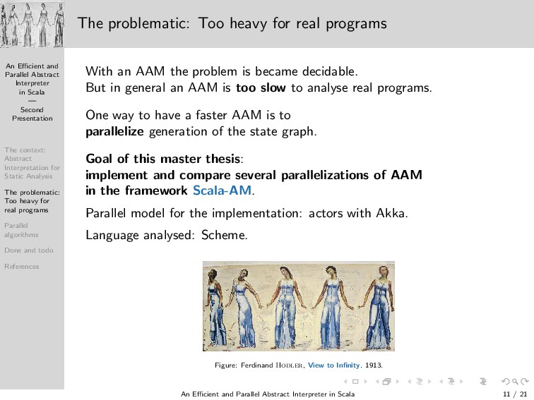
Presentation The context: Abstract Interpretation for Static Analysis The problematic: Too heavy for real programs Parallel algorithms Done and todo References The problematic: Too heavy for real programs With an AAM the problem is became decidable. But in general an AAM is too slow to analyse real programs. One way to have a faster AAM is to parallelize generation of the state graph. Goal of this master thesis: implement and compare several parallelizations of AAM in the framework Scala-AM. Parallel model for the implementation: actors with Akka. Language analysed: Scheme. Figure: Ferdinand Hodler, View to Infinity. 1913. An Efficient and Parallel Abstract Interpreter in Scala — Second Presentation 11 / 21
Presentation The context: Abstract Interpretation for Static Analysis The problematic: Too heavy for real programs Parallel algorithms Done and todo References 1 The context: Abstract Interpretation for Static Analysis 2 The problematic: Too heavy for real programs 3 Parallel algorithms 4 Done and todo 5 References An Efficient and Parallel Abstract Interpreter in Scala — Second Presentation 12 / 21
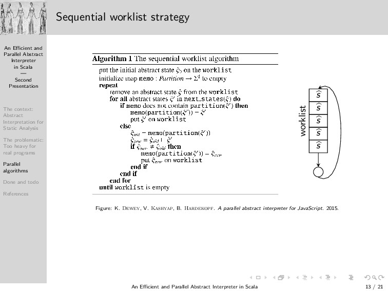
Presentation The context: Abstract Interpretation for Static Analysis The problematic: Too heavy for real programs Parallel algorithms Done and todo References Sequential worklist strategy s s s s s worklist Figure: K. Dewey, V. Kashyap, B. Hardekopf. A parallel abstract interpreter for JavaScript. 2015. An Efficient and Parallel Abstract Interpreter in Scala — Second Presentation 13 / 21
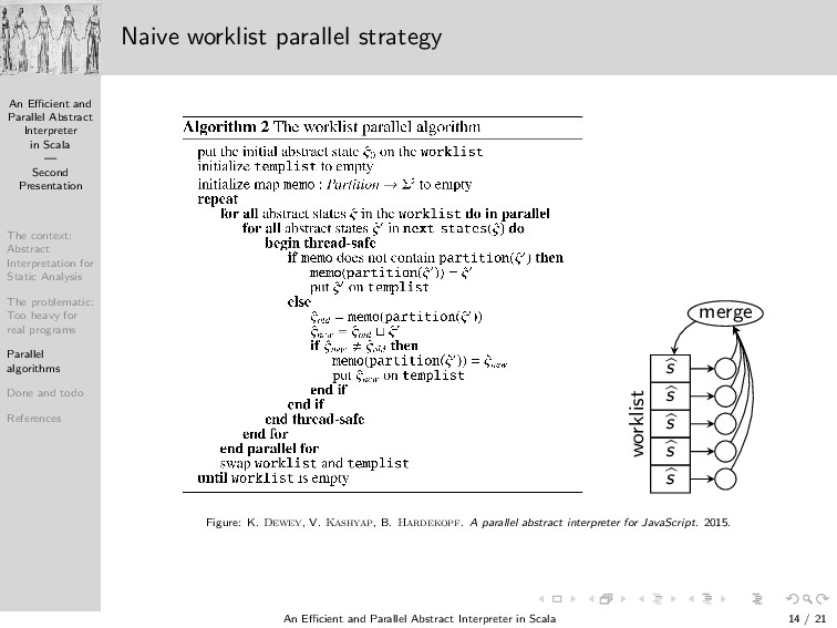
Presentation The context: Abstract Interpretation for Static Analysis The problematic: Too heavy for real programs Parallel algorithms Done and todo References Naive worklist parallel strategy s s s s s worklist merge Figure: K. Dewey, V. Kashyap, B. Hardekopf. A parallel abstract interpreter for JavaScript. 2015. An Efficient and Parallel Abstract Interpreter in Scala — Second Presentation 14 / 21
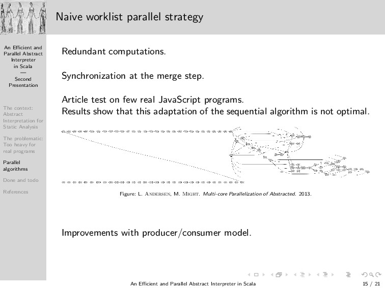
Presentation The context: Abstract Interpretation for Static Analysis The problematic: Too heavy for real programs Parallel algorithms Done and todo References Naive worklist parallel strategy Redundant computations. Synchronization at the merge step. Article test on few real JavaScript programs. Results show that this adaptation of the sequential algorithm is not optimal. Figure: L. Andersen, M. Might. Multi-core Parallelization of Abstracted. 2013. Improvements with producer/consumer model. An Efficient and Parallel Abstract Interpreter in Scala — Second Presentation 15 / 21
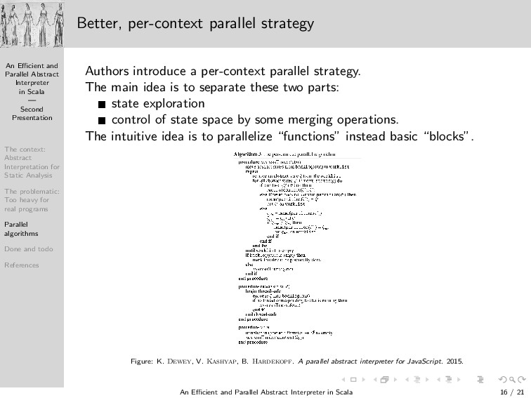
Presentation The context: Abstract Interpretation for Static Analysis The problematic: Too heavy for real programs Parallel algorithms Done and todo References Better, per-context parallel strategy Authors introduce a per-context parallel strategy. The main idea is to separate these two parts: state exploration control of state space by some merging operations. The intuitive idea is to parallelize “functions” instead basic “blocks”. Figure: K. Dewey, V. Kashyap, B. Hardekopf. A parallel abstract interpreter for JavaScript. 2015. An Efficient and Parallel Abstract Interpreter in Scala — Second Presentation 16 / 21
Presentation The context: Abstract Interpretation for Static Analysis The problematic: Too heavy for real programs Parallel algorithms Done and todo References 1 The context: Abstract Interpretation for Static Analysis 2 The problematic: Too heavy for real programs 3 Parallel algorithms 4 Done and todo 5 References An Efficient and Parallel Abstract Interpreter in Scala — Second Presentation 17 / 21
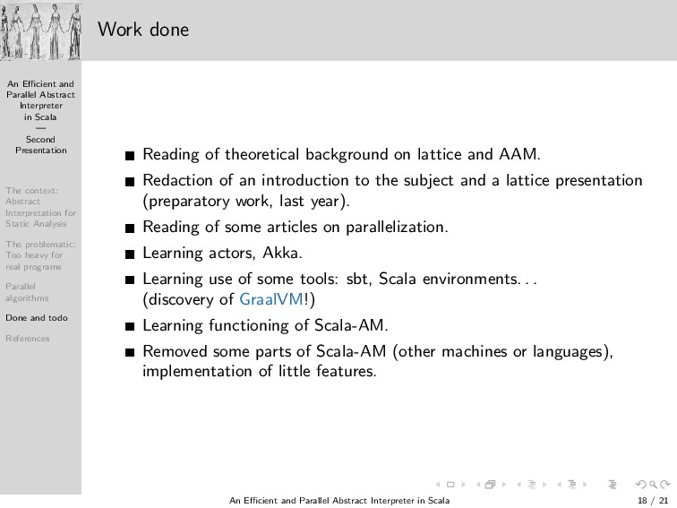
Presentation The context: Abstract Interpretation for Static Analysis The problematic: Too heavy for real programs Parallel algorithms Done and todo References Work done Reading of theoretical background on lattice and AAM. Redaction of an introduction to the subject and a lattice presentation (preparatory work, last year). Reading of some articles on parallelization. Learning actors, Akka. Learning use of some tools: sbt, Scala environments. . . (discovery of GraalVM!) Learning functioning of Scala-AM. Removed some parts of Scala-AM (other machines or languages), implementation of little features. An Efficient and Parallel Abstract Interpreter in Scala — Second Presentation 18 / 21
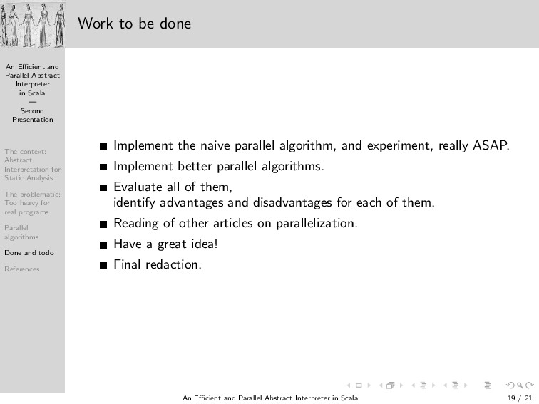
Presentation The context: Abstract Interpretation for Static Analysis The problematic: Too heavy for real programs Parallel algorithms Done and todo References Work to be done Implement the naive parallel algorithm, and experiment, really ASAP. Implement better parallel algorithms. Evaluate all of them, identify advantages and disadvantages for each of them. Reading of other articles on parallelization. Have a great idea! Final redaction. An Efficient and Parallel Abstract Interpreter in Scala — Second Presentation 19 / 21
Presentation The context: Abstract Interpretation for Static Analysis The problematic: Too heavy for real programs Parallel algorithms Done and todo References 1 The context: Abstract Interpretation for Static Analysis 2 The problematic: Too heavy for real programs 3 Parallel algorithms 4 Done and todo 5 References An Efficient and Parallel Abstract Interpreter in Scala — Second Presentation 20 / 21
Presentation The context: Abstract Interpretation for Static Analysis The problematic: Too heavy for real programs Parallel algorithms Done and todo References References Thank you! Questions time. . . L. Andersen, M. Might. Multi-core Parallelization of Abstracted Abstract Machines. 2013. Patrick Cousot. Abstract Interpretation in a Nutshell. K. Dewey, V. Kashyap, B. Hardekopf. A parallel abstract interpreter for JavaScript. 2015. Matthew Might. Tutorial: Small-step CFA. 2011. Quentin Sti´ evenart. Static Analysis of Concurrency Constructs in Higher-Order Programs. 2014. D. Van Horn, M. Might. Abstracting Abstract Machines. 2010. Document, L A TEX sources, complete references and first presentation on https:// Ø Ù ØºÓÖ »ÇÈ Å /efficient-parallel-abstract-interpreter-in-scala Olivier Pirson. An Efficient and Parallel Abstract Interpreter in Scala — Preparatory Work. 2017. An Efficient and Parallel Abstract Interpreter in Scala — Second Presentation 21 / 21