Modeling the Spatial Distribution of Hail Damage in Pine Plantations of Northern Spain as a Major Risk Factor for Forest Disease

Master thesis slides presented at LIFE Healthy Forest Project Meeting on Nov 7 2016, Vitoria (Spain)

Transcript

1. Modeling the Spatial Distribution of Hail Damage in Pine Plantations of Northern Spain as a Major Risk Factor for Forest Disease Patrick Schratz (patrick.schratz@uni-jena.de) November 7, 2016 Department of GIScience, University of Jena
2. “ Conducting data analysis is like drinking a fine wine. It is important to swirl and sniff the wine, to unpack the complex bouquet and to appreciate the experience. Gulping the wine doesn’t work. ” Daniel B. Wright, 2003 P. Schratz November 7, 2016 1 / 36
3. Introduction
4. Introduction Motivation: • Commercial pine plantations in northern Spain are affected by invasive pathogenic agents such as Diplodia pinea, Fusarium circinatum or Mycosphaerella spp. P. Schratz November 7, 2016 2 / 36
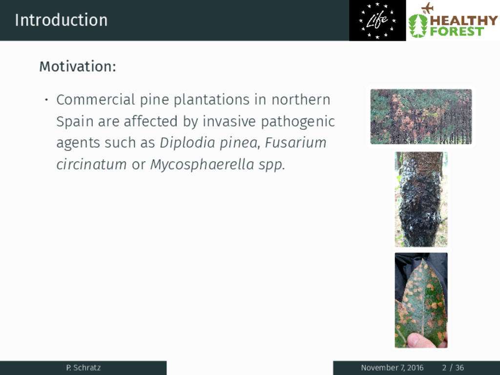
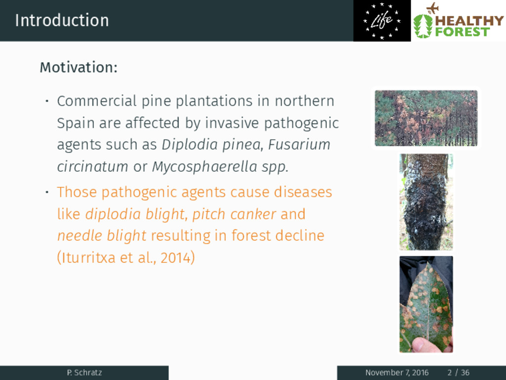
5. Introduction Motivation: • Commercial pine plantations in northern Spain are affected by invasive pathogenic agents such as Diplodia pinea, Fusarium circinatum or Mycosphaerella spp. • Those pathogenic agents cause diseases like diplodia blight, pitch canker and needle blight resulting in forest decline (Iturritxa et al., 2014) P. Schratz November 7, 2016 2 / 36
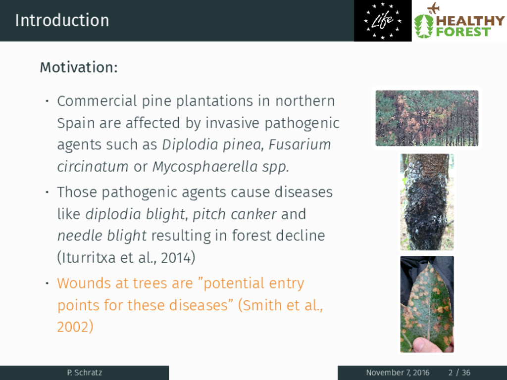
6. Introduction Motivation: • Commercial pine plantations in northern Spain are affected by invasive pathogenic agents such as Diplodia pinea, Fusarium circinatum or Mycosphaerella spp. • Those pathogenic agents cause diseases like diplodia blight, pitch canker and needle blight resulting in forest decline (Iturritxa et al., 2014) • Wounds at trees are ”potential entry points for these diseases” (Smith et al., 2002) P. Schratz November 7, 2016 2 / 36
7. Introduction Hypothesis: • (Severe) hail causes wounds favoring the nesting of pathogenic agents and subsequently forest decline P. Schratz November 7, 2016 3 / 36
8. Introduction Hypothesis: • (Severe) hail causes wounds favoring the nesting of pathogenic agents and subsequently forest decline Approach of this study: • Link surveyed ”hail damage to trees” to environmental variables to improve the understanding of forest decline in the Basque Country P. Schratz November 7, 2016 3 / 36
9. Introduction Hypothesis: • (Severe) hail causes wounds favoring the nesting of pathogenic agents and subsequently forest decline Approach of this study: • Link surveyed ”hail damage to trees” to environmental variables to improve the understanding of forest decline in the Basque Country • Usage of linear and non-linear statistical learning methods to identify risk areas of hail damage to trees P. Schratz November 7, 2016 3 / 36
10. Data and study area
11. Outline 1. Introduction 2. Data and study area 2.1. Study area 2.2. Data 3. Methods 4. Results 5. Conclusion P. Schratz November 7, 2016 4 / 36
12. Study area Figure 1: Spatial distribution of survey trees and species information P. Schratz November 7, 2016 5 / 36
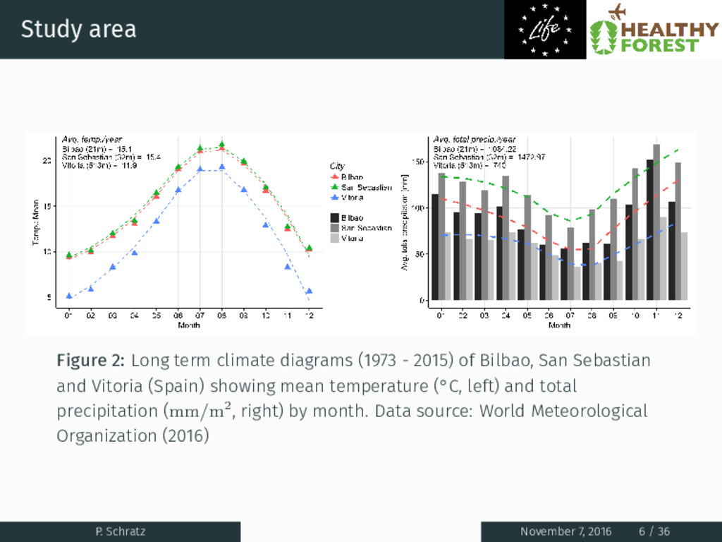
13. Study area Figure 2: Long term climate diagrams (1973 - 2015) of Bilbao, San Sebastian and Vitoria (Spain) showing mean temperature (°C, left) and total precipitation (mm/m2, right) by month. Data source: World Meteorological Organization (2016) P. Schratz November 7, 2016 6 / 36
14. Outline 1. Introduction 2. Data and study area 2.1. Study area 2.2. Data 3. Methods 4. Results 5. Conclusion P. Schratz November 7, 2016 7 / 36
15. Data Tree Survey Data Set (TSD) • 1168 observations • 2009-2012 P. Schratz November 7, 2016 8 / 36
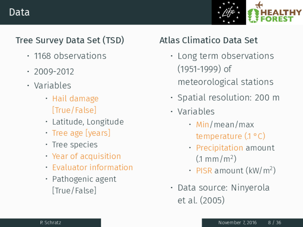
16. Data Tree Survey Data Set (TSD) • 1168 observations • 2009-2012 • Variables • Hail damage [True/False] • Latitude, Longitude • Tree age [years] • Tree species • Year of acquisition • Evaluator information • Pathogenic agent [True/False] P. Schratz November 7, 2016 8 / 36
17. Data Tree Survey Data Set (TSD) • 1168 observations • 2009-2012 • Variables • Hail damage [True/False] • Latitude, Longitude • Tree age [years] • Tree species • Year of acquisition • Evaluator information • Pathogenic agent [True/False] Atlas Climatico Data Set • Long term observations (1951-1999) of meteorological stations • Spatial resolution: 200 m P. Schratz November 7, 2016 8 / 36
18. Data Tree Survey Data Set (TSD) • 1168 observations • 2009-2012 • Variables • Hail damage [True/False] • Latitude, Longitude • Tree age [years] • Tree species • Year of acquisition • Evaluator information • Pathogenic agent [True/False] Atlas Climatico Data Set • Long term observations (1951-1999) of meteorological stations • Spatial resolution: 200 m • Variables • Min/mean/max temperature (.1 °C) • Precipitation amount (.1 mm/m2) • PISR amount (kW/m2) • Data source: Ninyerola et al. (2005) P. Schratz November 7, 2016 8 / 36
19. Data Global Summary of [the] Day Product (GSOD) • 43 years of daily observations • Stations • Bilbao • San Sebastian • Vitoria • Data source: World Meteorological Organization (2016) P. Schratz November 7, 2016 9 / 36
20. Data Global Summary of [the] Day Product (GSOD) • 43 years of daily observations • Stations • Bilbao • San Sebastian • Vitoria • Data source: World Meteorological Organization (2016) • Variables • Min/mean/max temperature (.1 Fahrenheit) • Mean wind speed (.1 knots) • Precipitation amount (.01 inches) • Occurrence of hail P. Schratz November 7, 2016 9 / 36
21. Data Global Summary of [the] Day Product (GSOD) • 43 years of daily observations • Stations • Bilbao • San Sebastian • Vitoria • Data source: World Meteorological Organization (2016) • Variables • Min/mean/max temperature (.1 Fahrenheit) • Mean wind speed (.1 knots) • Precipitation amount (.01 inches) • Occurrence of hail Digital Elevation Model • Spatial resolution: 25 m • Point density: 2 points/m • Data source: Euskadi (2013) P. Schratz November 7, 2016 9 / 36
22. Methods
23. Workflow I P. Schratz November 7, 2016 10 / 36
24. Workflow II P. Schratz November 7, 2016 11 / 36
25. GL(M)M & GA(M)M Model Setup Model Specification • Response • Hail damage to trees • Type ’binomial’ -> Logit link function P. Schratz November 7, 2016 12 / 36
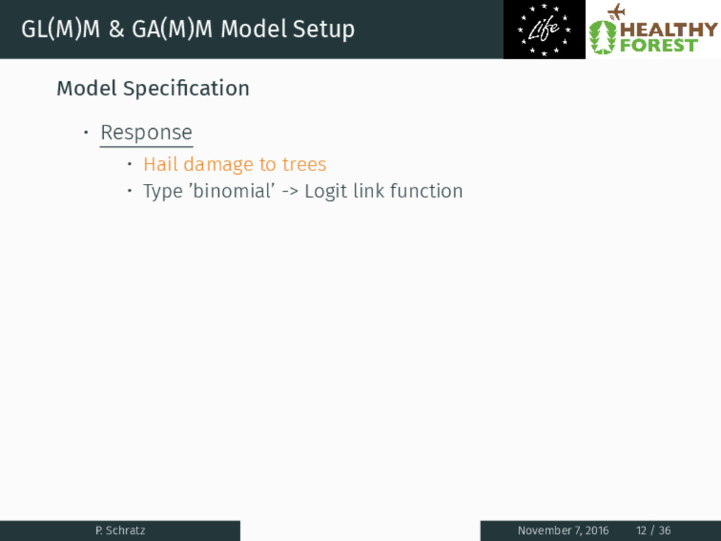
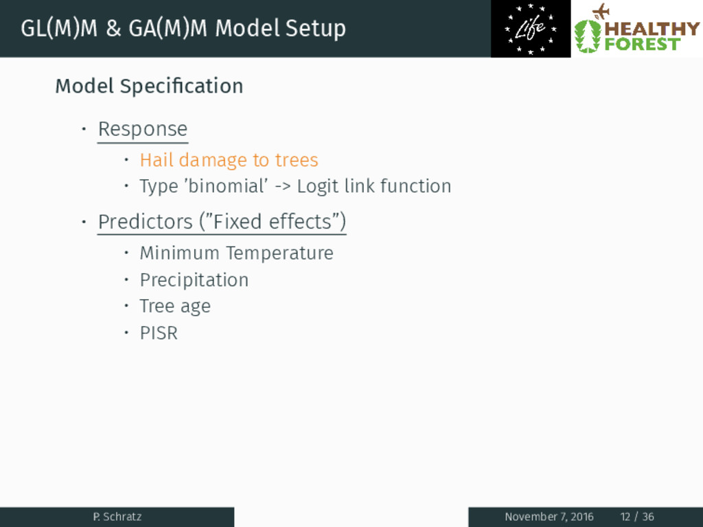
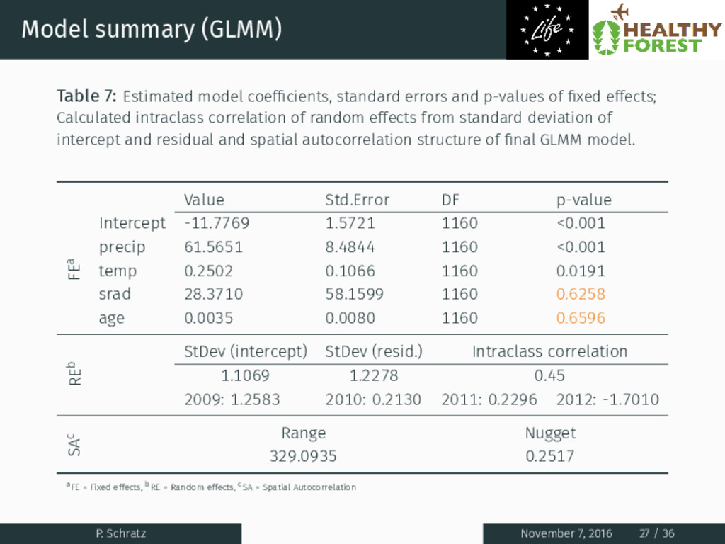
26. GL(M)M & GA(M)M Model Setup Model Specification • Response • Hail damage to trees • Type ’binomial’ -> Logit link function • Predictors (”Fixed effects”) • Minimum Temperature • Precipitation • Tree age • PISR P. Schratz November 7, 2016 12 / 36
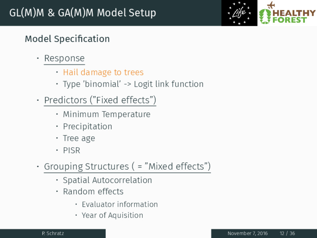
27. GL(M)M & GA(M)M Model Setup Model Specification • Response • Hail damage to trees • Type ’binomial’ -> Logit link function • Predictors (”Fixed effects”) • Minimum Temperature • Precipitation • Tree age • PISR • Grouping Structures ( = ”Mixed effects”) • Spatial Autocorrelation • Random effects • Evaluator information • Year of Aquisition P. Schratz November 7, 2016 12 / 36
28. Results
29. Outline 1. Introduction 2. Data and study area 3. Methods 4. Results 4.1. Synoptic Weather Situation Related to Hail Occurence 4.2. Statistical Modelling 5. Conclusion P. Schratz November 7, 2016 13 / 36
30. Synoptic Weather Situation Related to Hail Occurence Figure 3: Hail occurrences of Bilbao, San Sebastian and Vitoria for the years 1973 - 2015 P. Schratz November 7, 2016 14 / 36
31. Synoptic Weather Situation Related to Hail Occurence Figure 4: Hail occurrences of Bilbao, San Sebastian and Vitoria by month for the time period 1973 - 2015 P. Schratz November 7, 2016 15 / 36
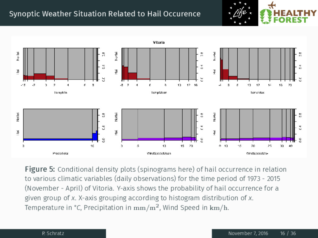
32. Synoptic Weather Situation Related to Hail Occurence Figure 5: Conditional density plots (spinograms here) of hail occurrence in relation to various climatic variables (daily observations) for the time period of 1973 - 2015 (November - April) of Vitoria. Y-axis shows the probability of hail occurrence for a given group of x. X-axis grouping according to histogram distribution of x. Temperature in °C, Precipitation in mm/m2, Wind Speed in km/h. P. Schratz November 7, 2016 16 / 36
33. Outline 1. Introduction 2. Data and study area 3. Methods 4. Results 4.1. Synoptic Weather Situation Related to Hail Occurence 4.2. Statistical Modelling 5. Conclusion P. Schratz November 7, 2016 17 / 36
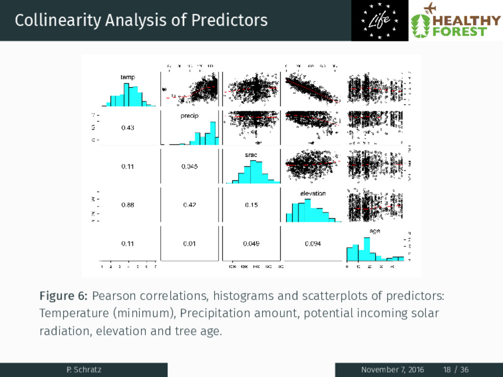
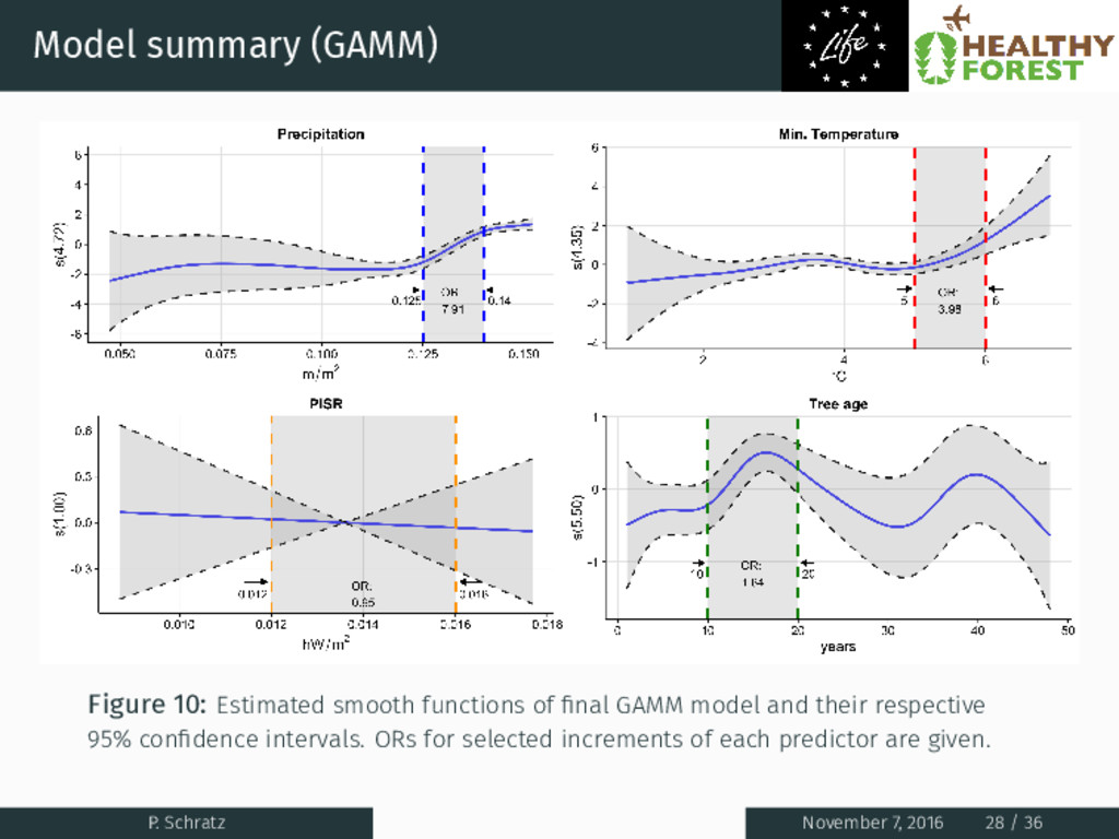
34. Collinearity Analysis of Predictors Figure 6: Pearson correlations, histograms and scatterplots of predictors: Temperature (minimum), Precipitation amount, potential incoming solar radiation, elevation and tree age. P. Schratz November 7, 2016 18 / 36
35. Collinearity Analysis of Predictors Table 1: Variance Inflation Factors (VIF) of all predictors (with and without elevation) temp precip srad age elevation VIF (with elevation) 4.11 1.04 1.38 1.00 3.96 VIF (without elevation) 1.07 1.03 1.04 1.00 - P. Schratz November 7, 2016 19 / 36
36. Descriptive Summaries of Non-Numerical Variables Table 2: Descriptive summary statistics of non-numerical variables Variable Levels n % ∑ % year 2009 494 42.3 42.3 2010 330 28.2 70.5 2011 143 12.2 82.8 2012 201 17.2 100.0 all 1168 100.0 evaluation 1 1048 89.7 89.7 2 120 10.3 100.0 all 1168 100.0 hail 0 929 79.5 79.5 1 239 20.5 100.0 all 1168 100.0 P. Schratz November 7, 2016 20 / 36
37. Model setups Table 3: Overview of GLM & GLMM model setups Index Type RE SA 1 GLM - - 2 GLMM - + 3 GLMM Year - 4 GLMM Eval - 5 GLMM Year/Eval - 6 GLMM Year + Table 4: Overview of GAM & GAMM model setups Index Type RE SA Note 1 GAM - - 2 GAMM - + 3 GAMM Year + *DNC 4 GAMM Eval + *DNC 5 GAMM Year/Eval + *DNC 6 GAMM Year - 7 GAMM Eval - 8 GAMM Year/Eval - *DNC = Did Not Converge P. Schratz November 7, 2016 21 / 36
38. Spatial Autocorrelation (GLM) Before accounting Figure 7: Residual semivariogram of GLM (1) SVGM stats Range: 1911 m Nugget: 0.03 P. Schratz November 7, 2016 22 / 36
39. Spatial Autocorrelation (GLM) After accounting Figure 8: Pearson residual semivariogram of GLMM (2) SVGM stats Range: 83000 m Nugget: 0.4 P. Schratz November 7, 2016 23 / 36
40. Spatial Autocorrelation (GAM) Before accounting Figure 9: Pearson residual semivariogram of GAM (1) SVGM stats Range: 5024 m Nugget: 0.25 P. Schratz November 7, 2016 24 / 36
41. Spatial Autocorrelation (GAM) After accounting Information Spatial GAMM models did not converge no SVGM ”after accounting” P. Schratz November 7, 2016 25 / 36
42. Random Effects GLMM Table 5: Random effect magnitudes of GLMM year evaluation year/evaluation Intercept Residual Intercept Residual Intercept Residual StdDev 1.13 1.84 0.44 1.23 0.00 1.84 Intraclass correlation 0.27 0.11 0 GAMM Table 6: Magnitude of random effects of GAMM year evaluation year/evaluation Intercept Residual Intercept Residual Intercept Residual StdDev 1.17 1 0.34 1 1.23 1 Intraclass correlation 0.58 0.1 0.6 P. Schratz November 7, 2016 26 / 36
43. Model summary (GLMM) Table 7: Estimated model coefficients, standard errors and p-values of fixed effects; Calculated intraclass correlation of random effects from standard deviation of intercept and residual and spatial autocorrelation structure of final GLMM model. Value Std.Error DF p-value FEa Intercept -11.7769 1.5721 1160 <0.001 precip 61.5651 8.4844 1160 <0.001 temp 0.2502 0.1066 1160 0.0191 srad 28.3710 58.1599 1160 0.6258 age 0.0035 0.0080 1160 0.6596 REb StDev (intercept) StDev (resid.) Intraclass correlation 1.1069 1.2278 0.45 2009: 1.2583 2010: 0.2130 2011: 0.2296 2012: -1.7010 SAc Range Nugget 329.0935 0.2517 aFE = Fixed effects, bRE = Random effects, cSA = Spatial Autocorrelation P. Schratz November 7, 2016 27 / 36
44. Model summary (GAMM) Figure 10: Estimated smooth functions of final GAMM model and their respective 95% confidence intervals. ORs for selected increments of each predictor are given. P. Schratz November 7, 2016 28 / 36
45. (Spatial) Cross-Validation P. Schratz November 7, 2016 29 / 36
46. Prediction P. Schratz November 7, 2016 30 / 36
47. Prediction P. Schratz November 7, 2016 31 / 36
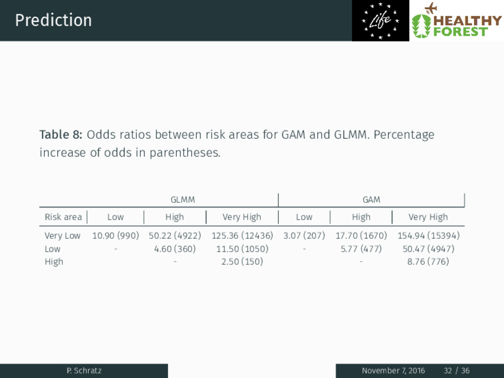
48. Prediction Table 8: Odds ratios between risk areas for GAM and GLMM. Percentage increase of odds in parentheses. GLMM GAM Risk area Low High Very High Low High Very High Very Low 10.90 (990) 50.22 (4922) 125.36 (12436) 3.07 (207) 17.70 (1670) 154.94 (15394) Low - 4.60 (360) 11.50 (1050) - 5.77 (477) 50.47 (4947) High - 2.50 (150) - 8.76 (776) P. Schratz November 7, 2016 32 / 36
49. Conclusion
50. Conclusion Synoptic weather situation of hail occurence • Prime time: November - April P. Schratz November 7, 2016 33 / 36
51. Conclusion Synoptic weather situation of hail occurence • Prime time: November - April • No long term increase of hail frequency P. Schratz November 7, 2016 33 / 36
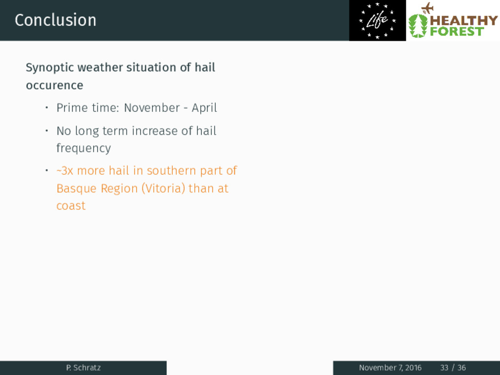
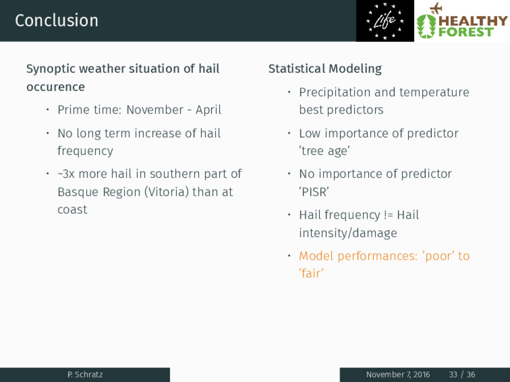
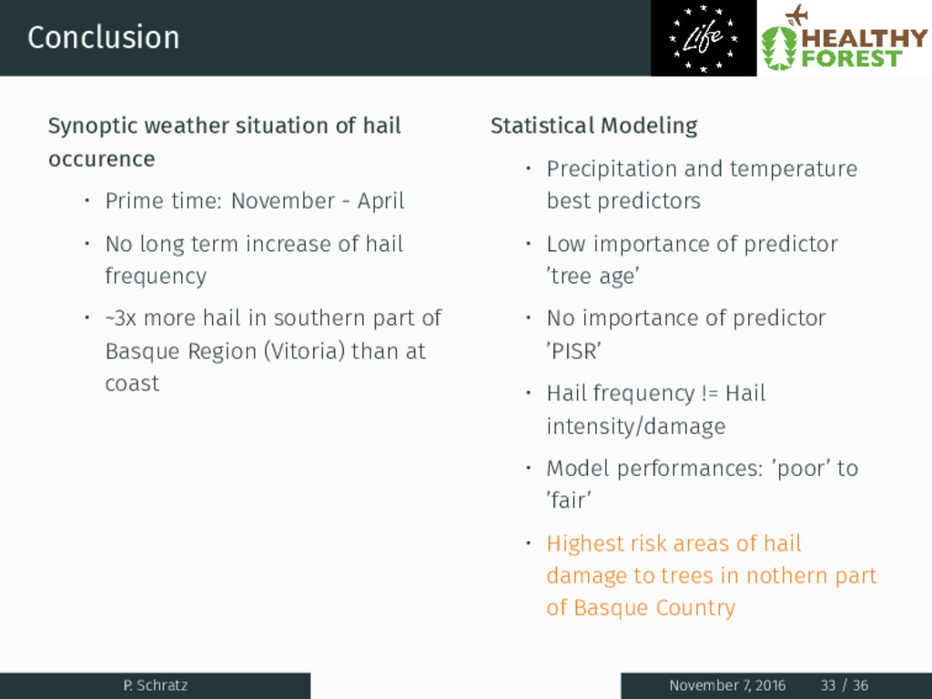
52. Conclusion Synoptic weather situation of hail occurence • Prime time: November - April • No long term increase of hail frequency • ~3x more hail in southern part of Basque Region (Vitoria) than at coast P. Schratz November 7, 2016 33 / 36
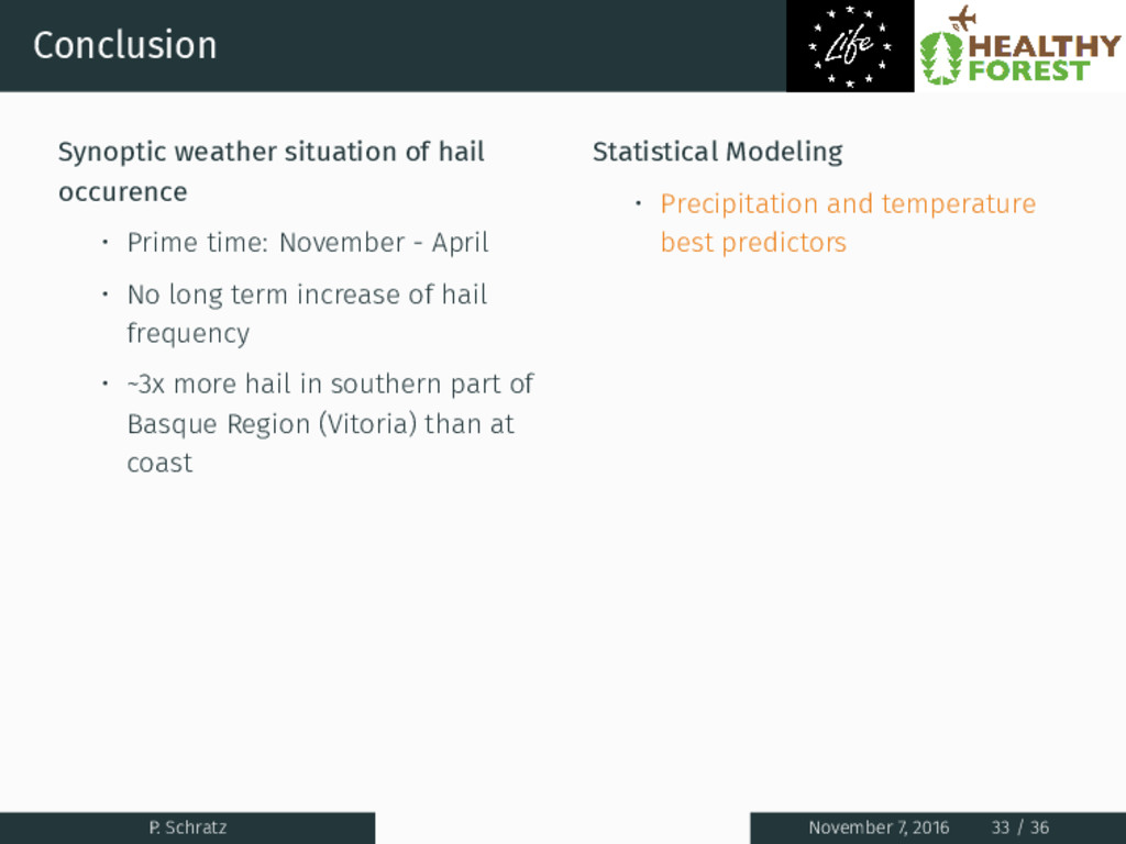
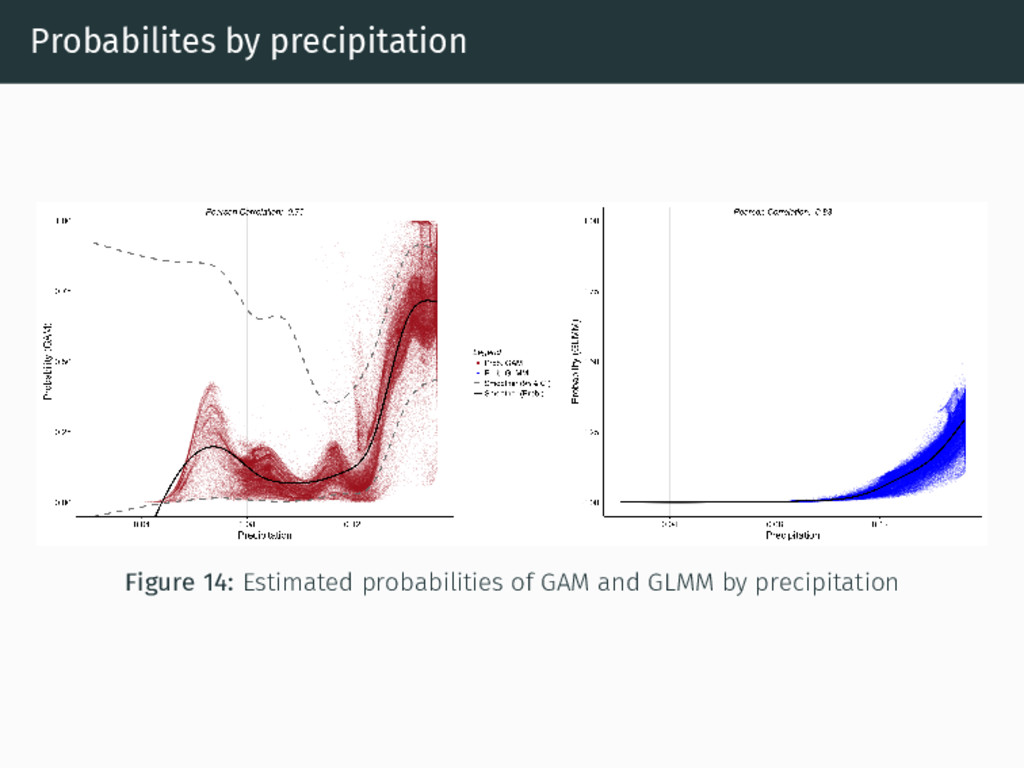
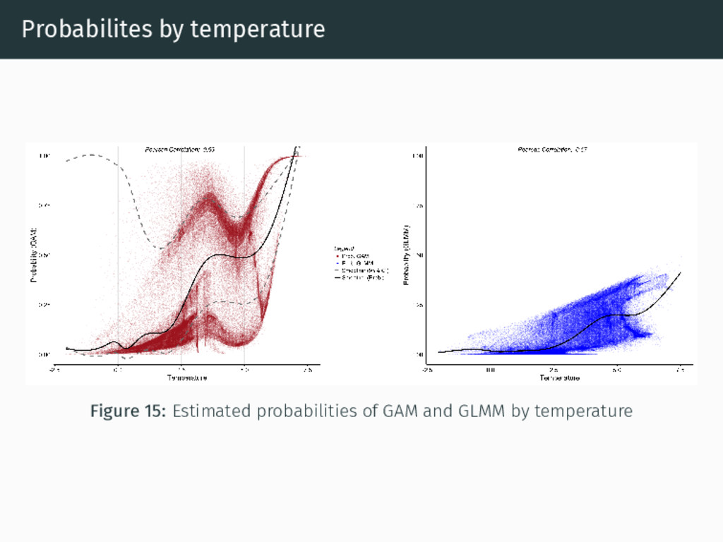
53. Conclusion Synoptic weather situation of hail occurence • Prime time: November - April • No long term increase of hail frequency • ~3x more hail in southern part of Basque Region (Vitoria) than at coast Statistical Modeling • Precipitation and temperature best predictors P. Schratz November 7, 2016 33 / 36
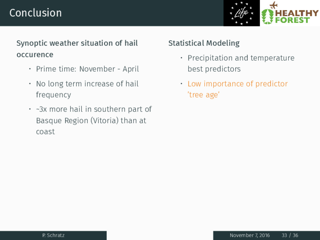
54. Conclusion Synoptic weather situation of hail occurence • Prime time: November - April • No long term increase of hail frequency • ~3x more hail in southern part of Basque Region (Vitoria) than at coast Statistical Modeling • Precipitation and temperature best predictors • Low importance of predictor ’tree age’ P. Schratz November 7, 2016 33 / 36
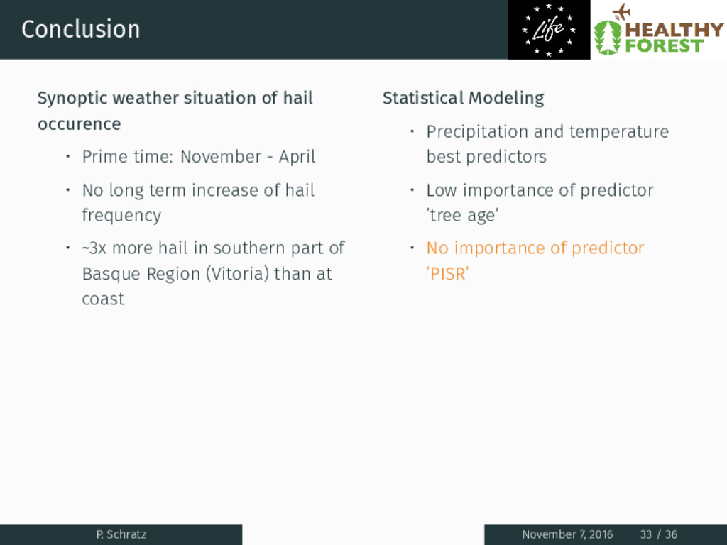
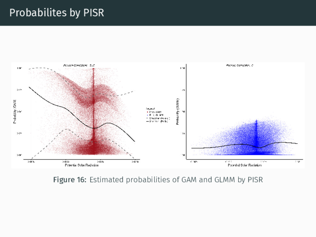
55. Conclusion Synoptic weather situation of hail occurence • Prime time: November - April • No long term increase of hail frequency • ~3x more hail in southern part of Basque Region (Vitoria) than at coast Statistical Modeling • Precipitation and temperature best predictors • Low importance of predictor ’tree age’ • No importance of predictor ’PISR’ P. Schratz November 7, 2016 33 / 36
56. Conclusion Synoptic weather situation of hail occurence • Prime time: November - April • No long term increase of hail frequency • ~3x more hail in southern part of Basque Region (Vitoria) than at coast Statistical Modeling • Precipitation and temperature best predictors • Low importance of predictor ’tree age’ • No importance of predictor ’PISR’ • Hail frequency != Hail intensity/damage P. Schratz November 7, 2016 33 / 36
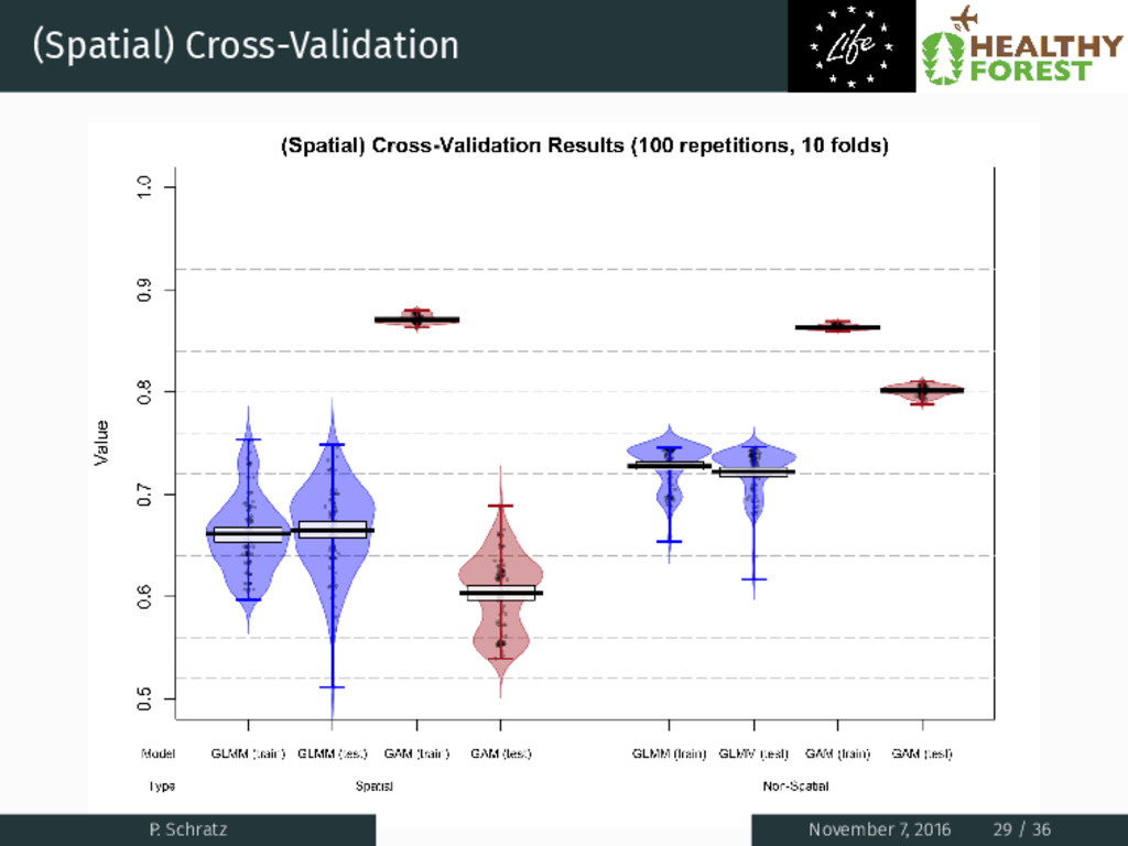
57. Conclusion Synoptic weather situation of hail occurence • Prime time: November - April • No long term increase of hail frequency • ~3x more hail in southern part of Basque Region (Vitoria) than at coast Statistical Modeling • Precipitation and temperature best predictors • Low importance of predictor ’tree age’ • No importance of predictor ’PISR’ • Hail frequency != Hail intensity/damage • Model performances: ’poor’ to ’fair’ P. Schratz November 7, 2016 33 / 36
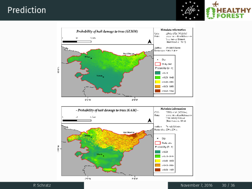
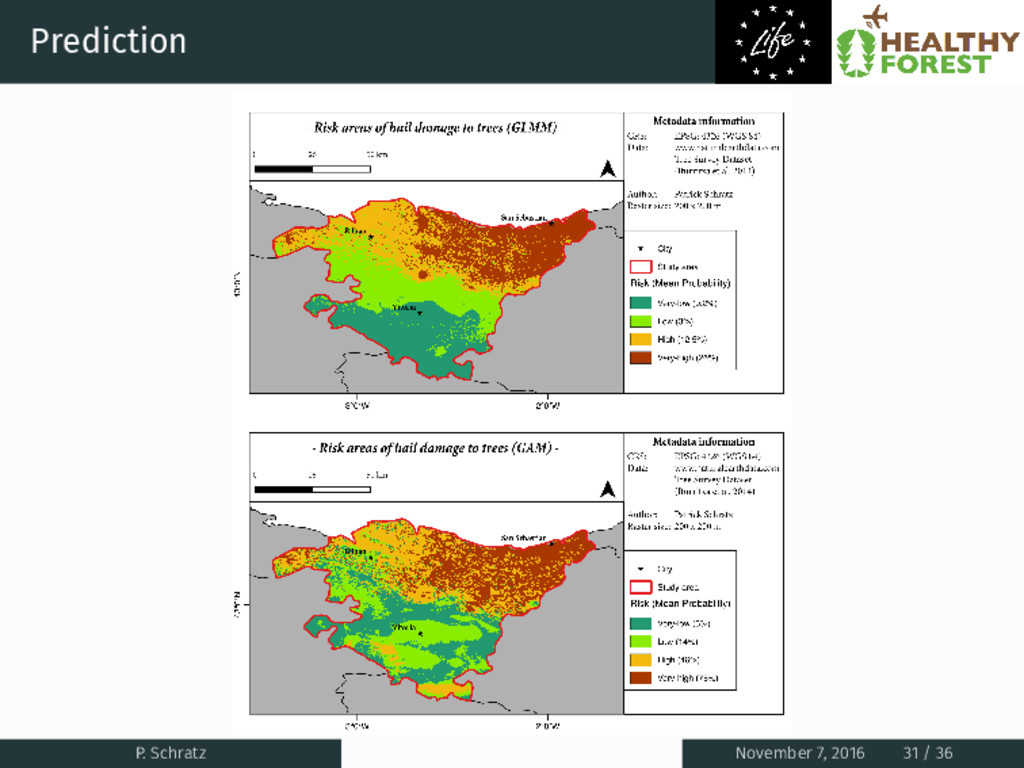
58. Conclusion Synoptic weather situation of hail occurence • Prime time: November - April • No long term increase of hail frequency • ~3x more hail in southern part of Basque Region (Vitoria) than at coast Statistical Modeling • Precipitation and temperature best predictors • Low importance of predictor ’tree age’ • No importance of predictor ’PISR’ • Hail frequency != Hail intensity/damage • Model performances: ’poor’ to ’fair’ • Highest risk areas of hail damage to trees in nothern part of Basque Country P. Schratz November 7, 2016 33 / 36
59. Future research • Apply concept to other study areas and compare results P. Schratz November 7, 2016 34 / 36
60. Future research • Apply concept to other study areas and compare results • Integrate more climatic variables (e.g. wind speed) P. Schratz November 7, 2016 34 / 36
61. Future research • Apply concept to other study areas and compare results • Integrate more climatic variables (e.g. wind speed) • Investigate non-convergence of spatial GAMM P. Schratz November 7, 2016 34 / 36
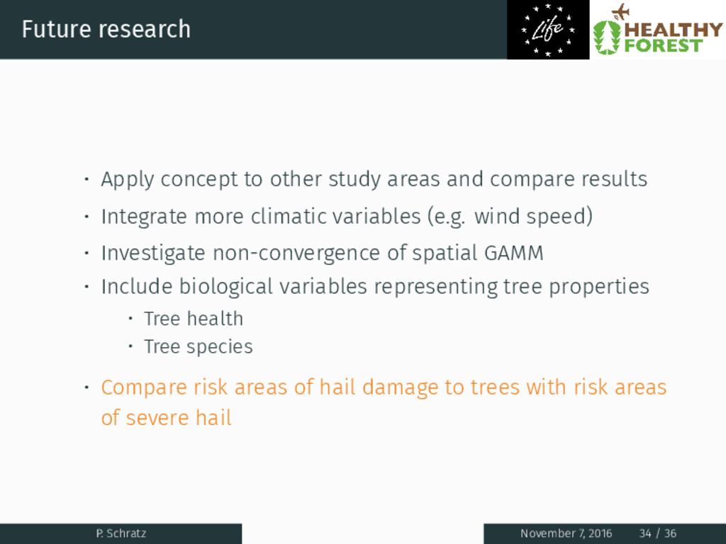
62. Future research • Apply concept to other study areas and compare results • Integrate more climatic variables (e.g. wind speed) • Investigate non-convergence of spatial GAMM • Include biological variables representing tree properties • Tree health • Tree species P. Schratz November 7, 2016 34 / 36
63. Future research • Apply concept to other study areas and compare results • Integrate more climatic variables (e.g. wind speed) • Investigate non-convergence of spatial GAMM • Include biological variables representing tree properties • Tree health • Tree species • Compare risk areas of hail damage to trees with risk areas of severe hail P. Schratz November 7, 2016 34 / 36
64. Bibliography I Brenning, A. (2012). Spatial cross-validation and bootstrap for the assessment of prediction rules in remote sensing: the R package sperrorest. In 2012 IEEE International Geoscience and Remote Sensing Symposium (pp. 5372–5375). doi:10.1109/IGARSS.2012.6352393 Euskadi. (2013). LiDAR based 25m digital elevation model of the Basque region. Retrieved from ftp://ftp.geo.euskadi.net/lidar Fielding, A. H. (2007). Cluster and classification techniques for the biosciences. Iturritxa, E., Mesanza, N., & Brenning, A. (2014). Spatial analysis of the risk of major forest diseases in Monterey pine plantations. Plant Pathology, 64(4), 880–889. doi:10.1111/ppa.12328 James, G., Witten, D., Hastie, T., & Tibshirani, R. (2013). An introduction to statistical learning. Springer. Ninyerola, M., Pons, X., & Roure, J. (2005). Atlas climático digital de lapenínsula ibérica. metodología y aplicaciones en bioclimatología y geobotánica. Universidad Autónoma de Barcelona, Bellaterra. P. Schratz November 7, 2016 35 / 36
65. Bibliography II Smith, H., Wingfield, M., & Coutinho, T. (2002). The role of latent Sphaeropsis Sapinea infections in post-hail associated die-back of Pinus Patula. Forest Ecology and Management, 164(1-3), 177–184. doi:10.1016/s0378-1127(01)00610-7 Snijders, T. & Bosker, R. (1991). An introduction to basic and advanced multilevel modelling. SAGE Publications Ltd, Thousand Oaks, CA. World Meteorological Organization. (2016). National Climatic Data Center (NCDC): Global Summary of [the] Day (GSOD) database [online accessed: 15/06/2016]. Retrieved from http://www7.ncdc.noaa.gov/CDO/cdoselect.cmd?datasetabbv= GSOD&countryabbv=&georegionabbv= Zuur, A. F., Ieno, E. N., Walker, N. J., Saveliev, A. A., & Smith, G. M. (2008). Mixed effects models and extensions in ecology with R. Springer. P. Schratz November 7, 2016 36 / 36
66. Thanks for your attention! Theme: metropolis - https://github.com/matze/mtheme (v1.1) Compilation: arara - https://github.com/cereda/arara (v3.0) Presentation mode: pdfpc - https://github.com/pdfpc/pdfpc (v.4.0.3) Created using the L ATEX beamer class P. Schratz November 7, 2016 36 / 36
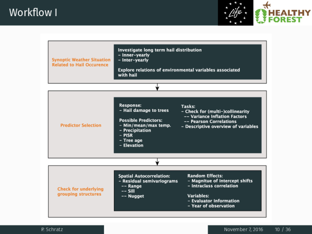
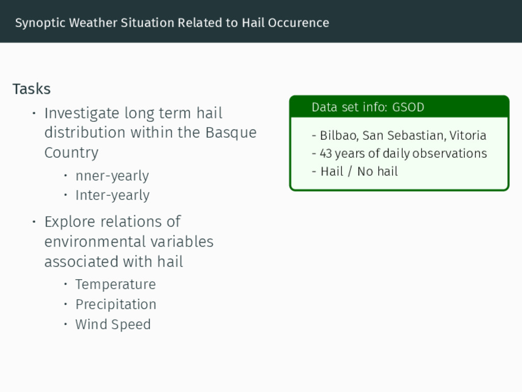
67. Synoptic Weather Situation Related to Hail Occurence Tasks • Investigate long term hail distribution within the Basque Country • nner-yearly • Inter-yearly • Explore relations of environmental variables associated with hail • Temperature • Precipitation • Wind Speed Data set info: GSOD - Bilbao, San Sebastian, Vitoria - 43 years of daily observations - Hail / No hail
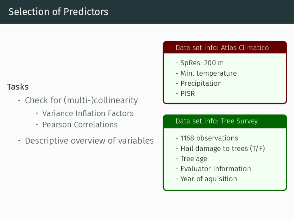
68. Selection of Predictors Tasks • Check for (multi-)collinearity • Variance Inflation Factors • Pearson Correlations • Descriptive overview of variables Data set info: Atlas Climatico - SpRes: 200 m - Min. temperature - Precipitation - PISR Data set info: Tree Survey - 1168 observations - Hail damage to trees (T/F) - Tree age - Evaluator information - Year of aquisition
69. Check for ”Mixed effects” Spatial Autocorrelation • Calculate residual semivariogram of GLM & GAM • Evaluate and account for sp. autocorrelation
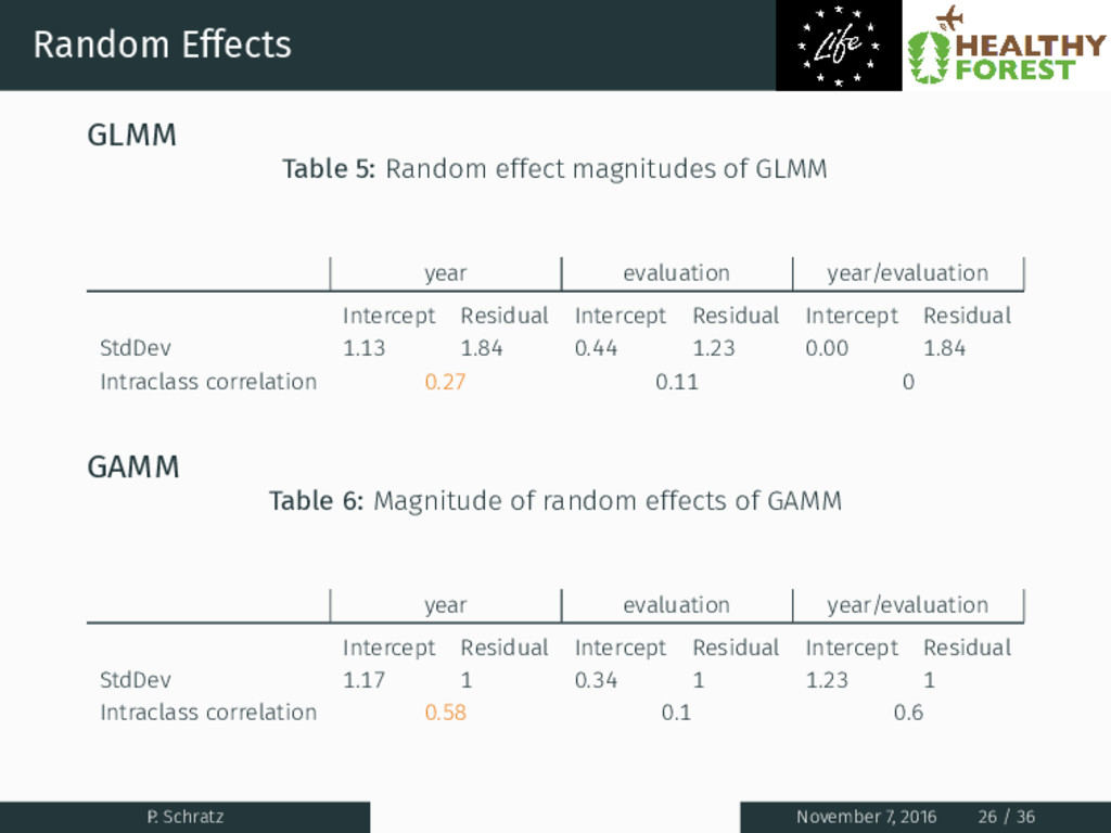
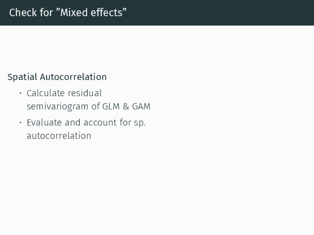
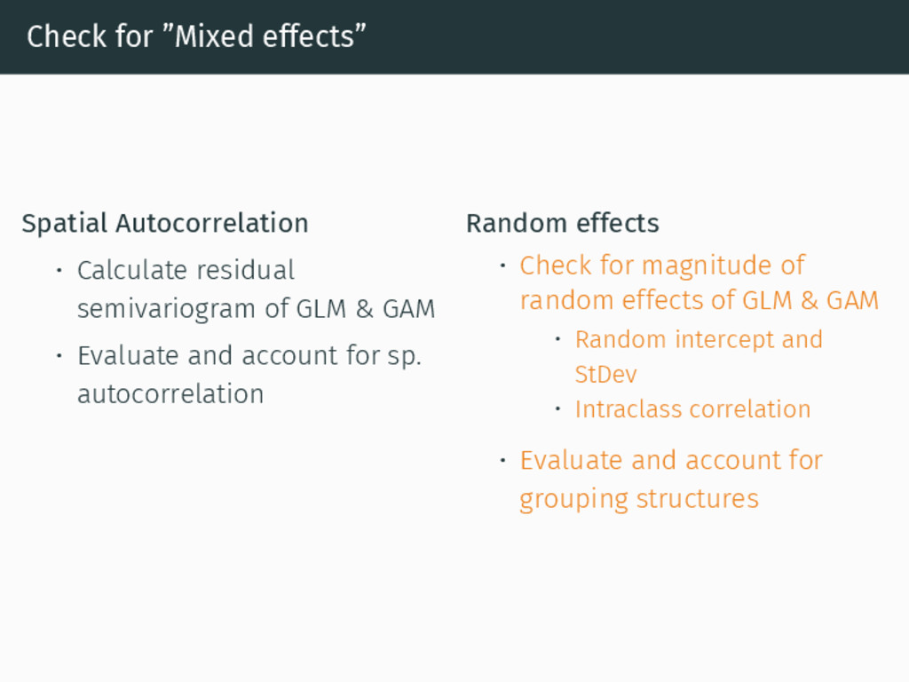
70. Check for ”Mixed effects” Spatial Autocorrelation • Calculate residual semivariogram of GLM & GAM • Evaluate and account for sp. autocorrelation Random effects • Check for magnitude of random effects of GLM & GAM • Random intercept and StDev • Intraclass correlation • Evaluate and account for grouping structures
71. (Spatial) Cross-Validation Cross-Validation setup • 100 repetitions, 10 folds • Spatial & non-spatial • GAM(M) + GL(M)M CV & AUROC Theory Figure 12: Schematic display of 5-fold cross-validation. Source: James et al. (2013) Spatial Cross-Validation Avoids too optimistic model performances (undetected overfitting) when sp. Autocor. is present (Brenning, 2012). Figure 13: Exemplary ROC curves. Source: Fielding (2007)
72. (Spatial) Cross-Validation Cross-Validation setup • 100 repetitions, 10 folds || Spatial & non-spatial || GAM(M) + GL(M)M Spatial CV Non-spatial CV
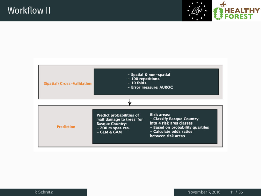
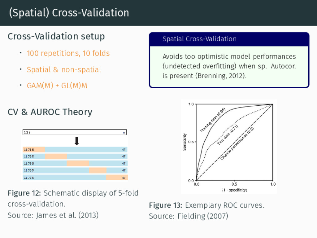
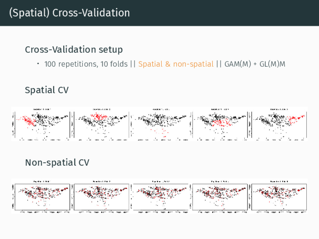
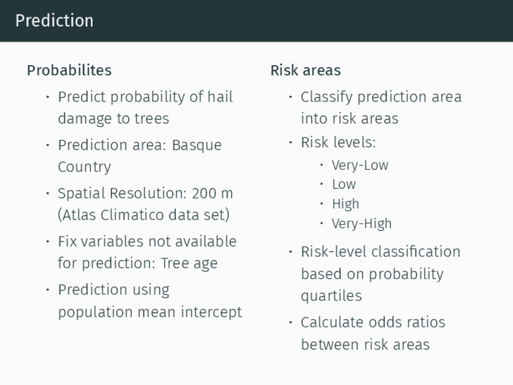
73. Prediction Probabilites • Predict probability of hail damage to trees • Prediction area: Basque Country • Spatial Resolution: 200 m (Atlas Climatico data set) • Fix variables not available for prediction: Tree age • Prediction using population mean intercept Risk areas • Classify prediction area into risk areas • Risk levels: • Very-Low • Low • High • Very-High • Risk-level classification based on probability quartiles • Calculate odds ratios between risk areas
74. Odds ratios GAM Table 9: Odds ratios for 20% increase intervals corresponding to the respective distribution quantile values of each predictor 0% - 20% 20% - 40% 40% - 60% 60% - 80% 80% - 100% value (precip) 0.047 - 0.068 0.068 - 0.089 0.089 - 0.11 0.11 - 0.131 0.131 - 0.152 OR (precip) 2.92 0.94 0.76 3.98 5.43 value (temp) 0.91 - 2.12 2.12 - 3.32 3.32 - 4.52 4.52 - 5.72 5.72 - 6.92 OR (temp) 1.57 1.93 0.68 2.39 17.67 value (srad) 0.009 - 0.01 0.01 - 0.012 0.012 - 0.014 0.014 - 0.016 0.016 - 0.018 OR (srad) 0.98 0.98 0.98 0.98 0.98 value (age) 1 - 10.4 10.4 - 19.8 19.8 - 29.2 29.2 - 38.6 38.6 - 48 OR (age) 1.37 1.61 0.46 1.90 0.44
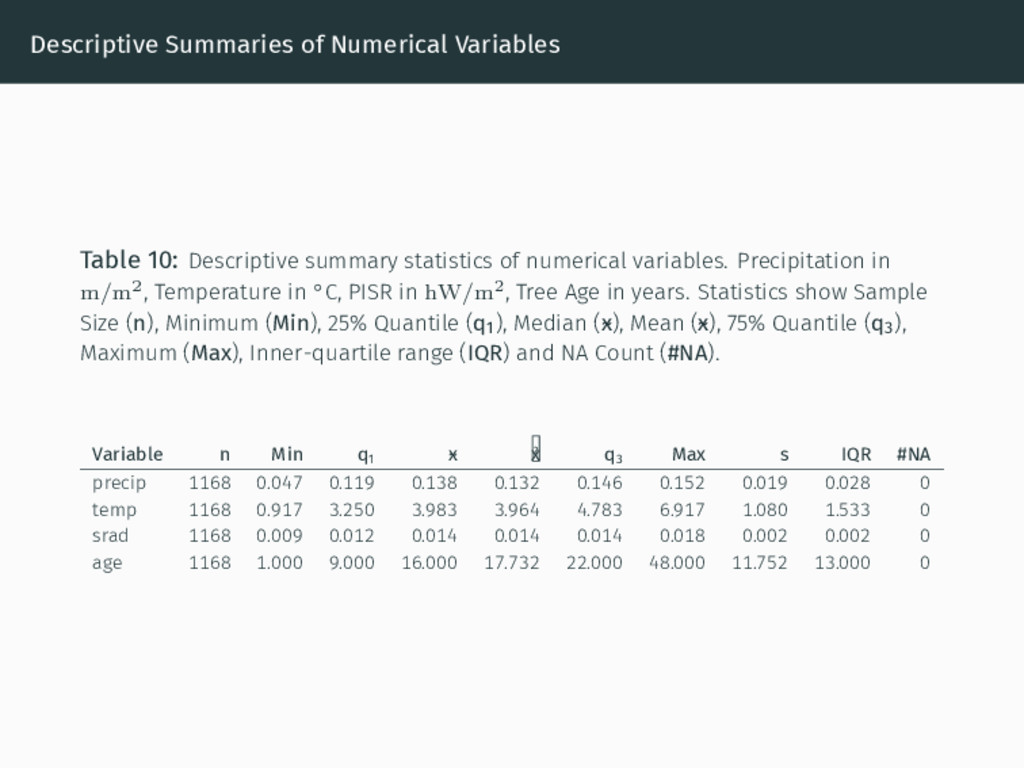
75. Descriptive Summaries of Numerical Variables Table 10: Descriptive summary statistics of numerical variables. Precipitation in m/m2, Temperature in °C, PISR in hW/m2, Tree Age in years. Statistics show Sample Size (n), Minimum (Min), 25% Quantile (q1 ), Median (~ x), Mean (~ x), 75% Quantile (q3 ), Maximum (Max), Inner-quartile range (IQR) and NA Count (#NA). Variable n Min q1 ~ x x q3 Max s IQR #NA precip 1168 0.047 0.119 0.138 0.132 0.146 0.152 0.019 0.028 0 temp 1168 0.917 3.250 3.983 3.964 4.783 6.917 1.080 1.533 0 srad 1168 0.009 0.012 0.014 0.014 0.014 0.018 0.002 0.002 0 age 1168 1.000 9.000 16.000 17.732 22.000 48.000 11.752 13.000 0
76. (Spatial) Cross-Validation Table 11: Descriptive statistics of (spatial) CV (10 folds, 100 repetitions) of GLMM and GAM GLMM GAM Spatial CV Non-Spatial CV Spatial CV Non-Spatial CV Train Test Train Test Train Test Train Test AUROC (median) 0.66 0.67 0.74 0.73 0.87 0.62 0.86 0.80 AUROC (StDev) 0.037 0.043 0.022 0.023 0.004 0.036 0.002 0.005
77. Probabilites by precipitation Figure 14: Estimated probabilities of GAM and GLMM by precipitation
78. Probabilites by temperature Figure 15: Estimated probabilities of GAM and GLMM by temperature
79. Probabilites by PISR Figure 16: Estimated probabilities of GAM and GLMM by PISR
80. Odds vs. Probability Two measures how likely an event may occur • odds = probability 1−probability • probability = odds 1+odds • Probability : [0, 1] • Odds : [−∞, +∞] Examples: • If the odds are 9:1 against you to reach the bus in time, this means you will miss the bus with a probability of 90% (in 9 of 10 cases). • Odds = 9/10 1−9/10 = 9 = 9:1 • Probability = 9/1 1+9/1 = 9 10 = 0.9
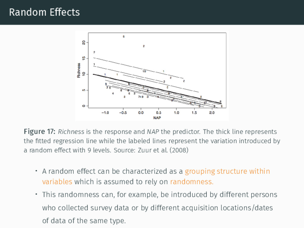
81. Random Effects Figure 17: Richness is the response and NAP the predictor. The thick line represents the fitted regression line while the labeled lines represent the variation introduced by a random effect with 9 levels. Source: Zuur et al. (2008) • A random effect can be characterized as a grouping structure within variables which is assumed to rely on randomness. • This randomness can, for example, be introduced by different persons who collected survey data or by different acquisition locations/dates of data of the same type.
82. Random Effects Intraclass/Induced Correlation • Intraclass correlation = Induced correlation (Snijders & Bosker, 1991) • Quantifies correlation among the random effect groups • The higher the correlation, the higher the need to account for the random effect structure in the model d2 d2+σ2 , where d is the intercept standard deviation and σ the standard deviation of the residuals of the random effect