Analyses bioinformatiques et statistiques de données de ChIP-seq sous UNIX et R - Support R Bioconductor

Transcript

1. Analyses bioinformatiques et statis- tiques de données ChIP-seq avec R / Bioconductor Pierre-François Roux 1 1pierre-francois.roux@ pasteur.fr 29 et 30 septembre 2016 Contents 1 Import des FASTQ et prétraitement des données . . . . 3 1.1 Import des FASTQ . . . . . . . . . . . . . . . . . . . . 3 1.2 Evaluer la qualité des FASTQ . . . . . . . . . . . . . . . 4 1.3 Filtrer et trimmer les FASTQ . . . . . . . . . . . . . . . 5 2 L’alignement . . . . . . . . . . . . . . . . . . . . . . . . . . 7 2.1 Téléchargement d’une référence FASTA. . . . . . . . . . 7 2.2 Manipulation des FASTA . . . . . . . . . . . . . . . . . 8 2.3 L’étape d’alignement . . . . . . . . . . . . . . . . . . . 9 2.4 Evaluer la qualité des alignements . . . . . . . . . . . . 9 3 Traitement des alignements . . . . . . . . . . . . . . . . . 10 3.1 Tri et indexation des BAM . . . . . . . . . . . . . . . . . 10 3.2 Travailler avec les BAM . . . . . . . . . . . . . . . . . . 10 4 La détection de pics . . . . . . . . . . . . . . . . . . . . . 12 4.1 Considérer les régions blacklistées . . . . . . . . . . . . 12 4.2 Estimer la taille des fragments . . . . . . . . . . . . . . 13 4.3 Compter les reads . . . . . . . . . . . . . . . . . . . . 13 4.4 Comparer les échantillons . . . . . . . . . . . . . . . . 15 5 Analyse différentielle . . . . . . . . . . . . . . . . . . . . . 16 5.1 Normalisation . . . . . . . . . . . . . . . . . . . . . . 16 5.2 Analyse différentielle avec edgeR . . . . . . . . . . . . . 17 5.3 Ajustement pour les tests multiples avec csaw . . . . . . . 18
2. Analyses bioinformatiques et statistiques de données ChIP-seq avec R / Bioconductor 5.4 Péparer les sorties BED et BIGWIG . . . . . . . . . . . . 19 6 Visualisation et interprétation fonctionnelle . . . . . . . . 19 6.1 Visualisation avec Gviz . . . . . . . . . . . . . . . . . . 19 6.2 Meta-profiles et heatmap . . . . . . . . . . . . . . . . . 20 2
3. Analyses bioinformatiques et statistiques de données ChIP-seq avec R / Bioconductor 1 Import des FASTQ et prétraitement des don- nées A chaque cylce de séquençage consistant en la succesion d’étapes d’incorpation de nucléotides, de lavages puis de lectures optiques, des images sont générées. Le signal ainsi obtenu est par la suite transformé en une information comprenant à la fois la succession nucléotidique ainsi que la qualité associée à chaque base. Cette information est la plupart du temps stockée sous le format FASTQ (FASTQ = FASTA + Qualité). Les informations relatives à la séquence nucléotidique et aux scores de qualité Phred sont encodées au format ASCII. Au final, l’information associée à un read occupe 4 lignes dans le fichier FASTQ. 1.1 Import des FASTQ Le package ShortRead propose des fonctions pemettant la manipulation de fichiers au format FASTQ dans R. Parmi les fonctions les plus utiles, mentionnons : • FastqSampler : permet de sélectionner aléatoirement un nombre défini de reads. • FastqStreamer : permet de parcourir un fichier FASTQ morceau par morceau. • readFastq : permet d’importer un fichier FASTQ dans R. Il est important de garder à l’esprit que les volumes de données manipulées peuvent être importants lorsque l’on travaille sur des données de séquençage. Aussi, les fonctions du type FastqStreamer permettant de découper les fichiers volumineux en sous-jeux de données de taille plus réduite sont à considérer dans les analyses à l’échelle du génome. Ici nous travaillons sur des données relatives à un chromosome uniquement, et pouvons nous permettre d’entrer la totalité des données en mémoire en utilisant readFastq . library(ShortRead) # Définir le répertoire de travail setwd("~/Documents/Enseignement/FC_AGRO_ChIPSeq_2016/Data/Jour_1/") # Lister les chemins d'accès aux fichiers FASTQ Fastq_Path <- dir("./", full=TRUE, pattern = "[12].fastq") # Lire les fcihiers FASTQ Fastq <- sapply(Fastq_Path, readFastq) L’objet ainsi créé est une liste de d’objets de classe ShortReadQ . Pour chaque FASTQ, les informations stockées sont les séquences nucléotidiques, les séquences de qualité Phred, et les identifiants des reads. Fastq[[1]] ## class: ShortReadQ ## length: 510192 reads; width: 36 cycles head(sread(Fastq[[1]]), 3) 3
4. Analyses bioinformatiques et statistiques de données ChIP-seq avec R / Bioconductor ## A DNAStringSet instance of length 3 ## width seq ## [1] 36 GTCGTGTGCGTTCCATTTTCCTAATGGAAAGTGGGG ## [2] 36 CATTTATCTCACACTCATAAGTGAGAACATGTGGTA ## [3] 36 GGAAACAACAGGCATTGGGGTCTACTTGAGGACGAT head(quality(Fastq[[1]]), 3) ## class: SFastqQuality ## quality: ## A BStringSet instance of length 3 ## width seq ## [1] 36 `a_[`U]`a^[^]_aaVaa`_aaaaaY[a[VU^]]X ## [2] 36 abbbbbbbbabaaaaaaaa``_aaaaaaaaa\]_[` ## [3] 36 `aaaaaba`aa___a``___\_a`_a``_]_\_a_` head(id(Fastq[[1]]), 3) ## A BStringSet instance of length 3 ## width seq ## [1] 35 ILLUMINA-EAS45_5:1:17:505:668:0:1:1 ## [2] 37 ILLUMINA-EAS45_5:1:38:1348:1833:0:1:1 ## [3] 35 ILLUMINA-EAS45_5:1:31:746:785:0:1:1 encoding(quality(Fastq[[1]])) ## ; < = > ? @ A B C D E F G H I J K L M N O P ## -5 -4 -3 -2 -1 0 1 2 3 4 5 6 7 8 9 10 11 12 13 14 15 16 ## Q R S T U V W X Y Z [ \\ ] ^ _ ` a b c d e f ## 17 18 19 20 21 22 23 24 25 26 27 28 29 30 31 32 33 34 35 36 37 38 ## g h i ## 39 40 41 alphabet(sread(Fastq[[1]])) ## [1] "A" "C" "G" "T" "M" "R" "W" "S" "Y" "K" "V" "H" "D" "B" "N" ## [16] "-" "+" "." 1.2 Evaluer la qualité des FASTQ Avant de procéder à des analyses plus approfondies, il est indispensable de procéder à l’analyse qualité des données brutes. Cette étape permet en e et d’évaluer rapidement si les runs de séquençage se sont déroulés correctement. Elle permet également d’évaluer si il est nécessaire de prétraiter les données butes avant de procéder à l’alignement. En dehors de l’environnement R , l’outil FastQC fait référence. Il génère cependant un rapport disctinct par FASTQ, ce qui ne facilite pas la comparaison entre échantillons. Le package Rqc consitue une solution idéale pour évaluer la qualité de données brutes relatives à des échantillons multiples et générer un rapport HTML. library(Rqc) # Générer les statistiques sur un échantillons de 100k reads QC_1 <- rqcQA(x = Fastq_Path, n = 100000, group = c(rep("ESR1_BP", 2), rep("ESR1_DMSO", 2))) P1 <- rqcCycleQualityBoxPlot(QC_1) P2 <- rqcCycleBaseCallsLinePlot(QC_1) 4
5. Analyses bioinformatiques et statistiques de données ChIP-seq avec R / Bioconductor ESR1_DMSO_REP1.fastq ESR1_DMSO_REP2.fastq ESR1_ES_REP1.fastq ESR1_ES_REP2.fastq 10 20 30 40 10 20 30 40 1 4 7 10 13 16 19 22 25 28 31 34 1 4 7 10 13 16 19 22 25 28 31 34 Cycle Quality Figure 1: Distribution de la qualité Phred par cycle - Données brutes ESR1_DMSO_REP1.fastq ESR1_DMSO_REP2.fastq ESR1_ES_REP1.fastq ESR1_ES_REP2.fastq 0 10 20 30 40 0 10 20 30 40 1 4 7 10 13 16 19 22 25 28 31 34 1 4 7 10 13 16 19 22 25 28 31 34 Cycle % Base Call A C G T N Figure 2: Fréquence (%) des bases par cycle - Données brutes 1.3 Filtrer et trimmer les FASTQ Au vu des résultats de l’analyse qualité, il est souvent nécessaire de pré-traiter les séquences brutes avant de procéder à l’alignement. Il est souvent recommandé de procéder à un filtre sur la quantité de bases non-assignées, sur la qualité Phred moyenne ou médiane, et parfois de retirer les bases situées à l’extrémité des reads. On parle alors de trimming statique. Comme nous pouvons le voir ici, certaines librairies sont clairement contaminées par des séquences d’adapteurs. Il est souhaitable de procéder à leur retrait et de procéder à un trimming dynamique. Cependant, l’environnement R ne s’y prète pas vraiment. D’autres outils développés en C++ ou Python comme Cutadap ou Trimmomatic s’y prètent beaucoup plus2 . Ici 2A noter que cette étape n’est pas indispensable puisque les adapteurs seront trimmés par l’aligneur si celui-ci est correctement paramétré 5
6. Analyses bioinformatiques et statistiques de données ChIP-seq avec R / Bioconductor nous adopterons une approche basique reposant sur le package QuasR , en retirant les reads contenant plus d’un N, en procédant à un trimming des séquences d’adapteurs basique peu paramétrable et biaisant les extrémités, puis en en retirant les reads d’une taille inférieure à 25. library("QuasR") # Préparer une fonction pour filtrer et trimmer les reads FilterAndTrim <- function(input_fq) { preprocessReads(input_fq, gsub(".fastq" ,"_TRIMMED.fastq", input_fq), nBases = 1, Lpattern = "AGATCGGAAGAG", Rpattern = "AGATCGGAAGAG", minLength = 25, truncateStartBases = 3, truncateEndBases = 3) } # Procéder au filtre et au trimming des reads sapply(Fastq_Path, FilterAndTrim) library(Rqc) # Générer les statistiques sur un échantillon de 100k reads QC_2 <- rqcQA(x = gsub(".fastq" ,"_TRIMMED.fastq", Fastq_Path), n = 100000) P1 <- rqcCycleQualityBoxPlot(QC_2) P2 <- rqcCycleBaseCallsLinePlot(QC_2) ESR1_DMSO_REP1_TRIMMED.fastq ESR1_DMSO_REP2_TRIMMED.fastq ESR1_ES_REP1_TRIMMED.fastq ESR1_ES_REP2_TRIMMED.fastq 10 20 30 40 10 20 30 40 1 4 7 10 13 16 19 22 25 28 1 4 7 10 13 16 19 22 25 28 Cycle Quality Figure 3: Distribution de la qualité Phred par cycle - Données trimmées et filtrées 6
7. Analyses bioinformatiques et statistiques de données ChIP-seq avec R / Bioconductor ESR1_DMSO_REP1_TRIMMED.fastq ESR1_DMSO_REP2_TRIMMED.fastq ESR1_ES_REP1_TRIMMED.fastq ESR1_ES_REP2_TRIMMED.fastq 0 10 20 30 40 0 10 20 30 40 1 4 7 10 13 16 19 22 25 28 1 4 7 10 13 16 19 22 25 28 Cycle % Base Call A C G T N Figure 4: Fréquence (%) des bases par cycle - Données trimmées et filtrées 2 L’alignement Une fois les séquences brutes de ChIP-seq prétraitées, il s’agit de les aligner contre un génome de référence. Il exite de nombreux algorithmes d’alignement adaptés aux séquences courtes d’ADN génomique ( Bowtie , Bowtie2 ou encore BWA étant les plus connus), la majorité d’entre eux étant accessibles depuis UNIX . Bien que certains packages R comme Rbowtie o rent la possibilité de faire appel à ces algorithmes depuis R , les possibilités sous R sont plus limitées. Le package Subread propose un ensemble de fonctions assez complet pour l’analyse de données NGS, et inclue notamment deux algorithmes d’alignement ( Subread et Subjunc ) basés sur une approche “seed-and-vote”. L’alignemet via Bowtie faisant référence pour l’anlyse de données de ChIP-seq, nous allons ici de nouveau faire appel au package QuasR basé sur le package Rbowtie . 2.1 Téléchargement d’une référence FASTA Les références au format FASTA peuvent être téléchargées depuis le serveur FTP d’Ensembl. Nous téléchargeons ici la séquence FASTA du chromosome 19 de l’assemblage GRCh38 du génome humain, aussi appelé hg38. FTP <- "ftp://ftp.ensembl.org/pub/release-85/fasta/homo_sapiens/dna/" # Télécharger la référence (version 'soft mask') FTP_SM <- paste(FTP, "Homo_sapiens.GRCh38.dna_sm.chromosome.19.fa.gz", sep = "") download.file(FTP_SM, destfile = paste("./", "Homo_sapiens.GRCh38.dna_sm.chromosome.19.fa.gz", sep = ""), method = "wget") # Télécharger la référence (version 'mask'') 7
8. Analyses bioinformatiques et statistiques de données ChIP-seq avec R / Bioconductor FTP_RM <- paste(FTP, "Homo_sapiens.GRCh38.dna_rm.chromosome.19.fa.gz", sep = "") download.file(FTP_RM, destfile = paste("./", "Homo_sapiens.GRCh38.dna_rm.chromosome.19.fa.gz", sep = ""), method = "wget") 2.2 Manipulation des FASTA Les fichiers de séquences simples de type FASTA peuvent être manipulés sous R à l’aide des fonctions proposées par le package Biostrings . library(Biostrings) Ref_SM_Path <- "Homo_sapiens.GRCh38.dna_sm.chromosome.19.fa.gz" Ref_RM_Path <- "Homo_sapiens.GRCh38.dna_rm.chromosome.19.fa.gz" # Importer un fichier FASTA Ref <- readDNAStringSet(c(Ref_SM_Path, Ref_RM_Path)) # Obtenir la proportion de chaque base alphabetFrequency(Ref, baseOnly = TRUE, as.prob = TRUE) ## A C G T other ## [1,] 0.25832325 0.23806120 0.23987895 0.26071946 0.003017148 ## [2,] 0.09431324 0.09746889 0.09789151 0.09431619 0.616010177 # Obtenir le contenu en GC letterFrequency(Ref, "CG", as.prob = TRUE) ## C|G ## [1,] 0.4779401 ## [2,] 0.1953604 # Obtenir une partie de la séquence (1) toString(Ref[[1]][90000:90050]) ## [1] "GAACTAAGGTAGTTATGAATAGAGCTAAAACTTAGGCAACACCATCCTGGA" toString(Ref[[2]][90000:90050]) ## [1] "GAACTAAGGTAGTTATGAATAGAGCTAANNNNNNNNNNNNNNNNNNNNNNN" # Obtenir une partie de la séquence (2) subseq(Ref[[1]], start = 90000, end = 90050) ## 51-letter "DNAString" instance ## seq: GAACTAAGGTAGTTATGAATAGAGCTAAAACTTAGGCAACACCATCCTGGA # Obtenir une partie de la séquence (3) Views(Ref[[1]], start = c(90000, 100000), end = c(90050,100050)) ## Views on a 58617616-letter DNAString subject ## subject: NNNNNNNNNNNNNNNNNNNNNNNNNNNN...NNNNNNNNNNNNNNNNNNNNNNNNNNN ## views: ## start end width ## [1] 90000 90050 51 [GAACTAAGGTAGTTATGAA...TAGGCAACACCATCCTGGA] ## [2] 100000 100050 51 [GTTTCTACCAAGAAAGCAT...GAAAGATCATTAAACTGGA] 8
9. Analyses bioinformatiques et statistiques de données ChIP-seq avec R / Bioconductor 2.3 L’étape d’alignement Il est possible de modifier un grand nombre de paramètres pour l’étape d’alignement pour tenir compte des spécificités des données sur lesquelles nous travaillons. Dans notre cas, la qualité Phred des données ENCODE téléchargées est encodée au format SOLEXA et il faut adapter l’alignement en conséquence. Par ailleurs les reads étant courts, nous n’autoriserons qu’un seul mismatch. Nous ne retiendrons également que les lectures alignées sans ambiguïté. library("QuasR") library("R.utils") # Lire le fichier décrivant les échantillons Samples_Path <- "SAMPLES_ESR1.txt" Samples <- read.table(Samples_Path, header = T) Samples ## FileName SampleName ## 1 ESR1_DMSO_REP1.fastq ESR1_DMSO_REP1 ## 2 ESR1_DMSO_REP2.fastq ESR1_DMSO_REP2 ## 3 ESR1_ES_REP1.fastq ESR1_ES_REP1 ## 4 ESR1_ES_REP2.fastq ESR1_ES_REP2 # Décompresser la référence gunzip("Homo_sapiens.GRCh38.dna_rm.chromosome.19.fa.gz", overwrite = T) # Procéder à l'alignement avec qAlign Align <- qAlign(sampleFile = Samples_Path, genome = "./Homo_sapiens.GRCh38.dna_rm.chromosome.19.fa", maxHits = 1, paired = "no", alignmentParameter = c("--solexa-quals"), splicedAlignment = FALSE) 2.4 Evaluer la qualité des alignements Le package QuasR permet, via la fonction alignmentStats , d’obtenir rapidement un aperçu du taux d’alignement et de générer un rapport PDF. # Obtenir les statitistique d'alignement alignmentStats(Align) ## seqlength mapped unmapped ## ESR1_DMSO_REP1:genome 58617616 149693 360499 ## ESR1_DMSO_REP2:genome 58617616 82053 303918 ## ESR1_ES_REP1:genome 58617616 162022 346932 ## ESR1_ES_REP2:genome 58617616 126954 331699 9
10. Analyses bioinformatiques et statistiques de données ChIP-seq avec R / Bioconductor 3 Traitement des alignements Une fois alignées, les séquences ainsi que leurs coordonnées sur le génome sont stockées au format SAM (Sequence Alignment/Map) ou en leur équivalent binaire, le format BAM, moins gourmand en ressources de stocakge. En dehors de R , ces fichiers peuvent être manipulés avec Samtools , Picard Tools , deepTools . . . Dans R , de nombreux packages permettent également de travailler sur ces fichiers. Nous utiliserons ici essentiellement : • Biostrings qui o re une interface R à Sammtools , BCFtools et tabix . • GenomicAlignments qui fournit de nombreux outils performants pour la manipu- lation des alignements sous R. 3.1 Tri et indexation des BAM Avant de pouvoir importer les BAM dans R , il est indispensable de les trier par coordonnées et de procéder à leur indexation. Ces deux étapes sont déjà prises en charges par la commande qAlign . Néanmoins, si cela avait été nécéssaire, voici comment procéder depuis R en utilisant le package Rsamtools . library("Rsamtools") # Lister les BAM Bam_Path <- dir("./", full=TRUE, pattern = ".bam$") # Procéder au tri for (i in 1:4) { sortBam(Bam_Path[i], gsub(".bam", "_SORT", Bam_Path)[i]) } # Lister les BAM triés Bam_Path <- dir("./", full=TRUE, pattern = "_SORT.bam$") # Procéder à l'indexation for (i in 1:4) { indexBam(Bam_Path[i]) } 3.2 Travailler avec les BAM Le volume des fichiers BAM étant souvent important, il n’est pas toujours possible ni souhaitable de les importer en totalité dans R et ce, pour optimiser les temps de calculs et d’analyse. Le package GenomicAlignments o rent de nombreuses possibilités pour consulter toute ou partie de l’information stockée dans les BAM. On peut ainsi se focaliser sur : • which : les alignements correspondant à une ou plusieurs régions particulières du génome définies via des objet de type GRanges ou GRangesList . 10
11. Analyses bioinformatiques et statistiques de données ChIP-seq avec R / Bioconductor • what : un type d’information particulier relatif aux alignements. • flag : sur les alignements répondant à certains critères renseignés dans le champ du bitwise flag . Ces informations sont stockées dans un objet de type ScanBamParam qu’il conviendra de définir avant d’interroger les BAM. # Définir la région d'intérêt Which <- GRanges(seqnames = "19", IRanges(start = 1, end = 58617616)) Which ## GRanges object with 1 range and 0 metadata columns: ## seqnames ranges strand ## <Rle> <IRanges> <Rle> ## [1] 19 [1, 58617616] * ## ------- ## seqinfo: 1 sequence from an unspecified genome; no seqlengths # Définir le type d'information à récupérer scanBamWhat() ## [1] "qname" "flag" "rname" "strand" ## [5] "pos" "qwidth" "mapq" "cigar" ## [9] "mrnm" "mpos" "isize" "seq" ## [13] "qual" "groupid" "mate_status" What <- c("mapq") # Définir les lectures à considérer Flag <- scanBamFlag(isPaired = NA, isProperPair = NA, isUnmappedQuery = NA, hasUnmappedMate = NA, isMinusStrand = NA, isMateMinusStrand = NA, isFirstMateRead = NA, isSecondMateRead = NA, isNotPrimaryRead = NA, isSecondaryAlignment = NA, isNotPassingQualityControls = NA, isDuplicate = NA) # Combiner les 3 informations Param <- ScanBamParam(which = Which, what = What, flag = Flag) # Interroger les alignements Bam_GA <- readGAlignments(Bam_Path[1], param = Param) Bam_GA ## GAlignments object with 149693 alignments and 1 metadata column: ## seqnames strand cigar qwidth start ## <Rle> <Rle> <character> <integer> <integer> ## [1] 19 + 36M 36 61264 ## [2] 19 - 36M 36 62555 ## [3] 19 - 36M 36 64512 ## [4] 19 + 36M 36 66491 ## [5] 19 + 36M 36 66981 ## ... ... ... ... ... ... ## [149689] 19 - 36M 36 58588265 ## [149690] 19 + 36M 36 58591258 ## [149691] 19 + 36M 36 58598416 ## [149692] 19 + 36M 36 58599223 ## [149693] 19 - 36M 36 58599229 ## end width njunc | mapq ## <integer> <integer> <integer> | <integer> ## [1] 61299 36 0 | 255 ## [2] 62590 36 0 | 255 11
12. Analyses bioinformatiques et statistiques de données ChIP-seq avec R / Bioconductor ## [3] 64547 36 0 | 255 ## [4] 66526 36 0 | 255 ## [5] 67016 36 0 | 255 ## ... ... ... ... . ... ## [149689] 58588300 36 0 | 255 ## [149690] 58591293 36 0 | 255 ## [149691] 58598451 36 0 | 255 ## [149692] 58599258 36 0 | 255 ## [149693] 58599264 36 0 | 255 ## ------- ## seqinfo: 1 sequence from an unspecified genome L’objet ainsi créé est de type GAlignments . Sa structure est très similaire à celle des GRanges et la plupart des fonctions adaptées au traitement des GRanges sont également adaptées aux GAlignements . # Interroger la position start des alignements start(Bam_GA)[1:5] ## [1] 61264 62555 64512 66491 66981 # Interroger la taille des alignements width(Bam_GA)[1:5] ## [1] 36 36 36 36 36 # Interroger le chromosome des alignements seqnames(Bam_GA)[1:5] ## factor-Rle of length 5 with 1 run ## Lengths: 5 ## Values : 19 ## Levels(1): 19 # Interroger la CIGAR line des alignements cigar(Bam_GA)[1:5] ## [1] "36M" "36M" "36M" "36M" "36M" 4 La détection de pics 4.1 Considérer les régions blacklistées library("rtracklayer") Chain <- "http://hgdownload.cse.ucsc.edu/goldenpath/hg19/liftOver/hg19ToHg38.over.chain.gz" download.file(Chain, destfile = "hg19ToHg38.over.chain.gz") gunzip("hg19ToHg38.over.chain.gz", "hg19ToHg38.over.chain", overwrite = TRUE) Chain <- import.chain("hg19ToHg38.over.chain") HG19_BL <- import("wgEncodeDacMapabilityConsensusExcludable.bed.gz") HG38_BL <- liftOver(x = HG19_BL, chain = Chain) HG38_BL <- unlist(HG38_BL) 12
13. Analyses bioinformatiques et statistiques de données ChIP-seq avec R / Bioconductor 4.2 Estimer la taille des fragments library(csaw) # Lister les BAM triés Bam_Path <- dir("./", full=TRUE, pattern = "_SORT.bam$") # Exclure les régions blacklistées Param <- readParam(discard = HG38_BL) # Définir une fonction pour estimer la taille des fragments Max_Delay <- 500 X_Cor_F <- function(bam) { correlateReads(bam.files = bam, cross = TRUE, max.dist = Max_Delay, param = Param) } # Estimer la taille des fragments X_Cor <- sapply(Bam_Path,X_Cor_F) colnames(X_Cor) <- Samples[,2] # Produire une sortie graphique library(reshape2) library(ggplot2) X_Cor_2 <- melt(X_Cor)[,c(2:3)] X_Cor_2$Delay <- rep(seq(0:Max_Delay), 4) colnames(X_Cor_2) <- c("Sample", "CCF", "Delay") FL_Plot <- ggplot(X_Cor_2, aes(x = Delay, y = CCF, color = Sample)) + geom_line() # Obtenir les maxima FL <- apply(X_Cor, 2, maximizeCcf) 4.3 Compter les reads # Count reads in 150 bp sliding windows Win_Data <- windowCounts(bam.files = Bam_Path, width = 150, ext = FL, param = Param, filter = 10) # Count reads in 2000 bp bins Win_Bckgd <- windowCounts(bam.files = Bam_Path, bin = TRUE, width = 2000, param = Param) # Compare the two data sets 13
14. Analyses bioinformatiques et statistiques de données ChIP-seq avec R / Bioconductor 0.00 0.05 0.10 0.15 0.20 0 100 200 300 400 500 Delay CCF Sample ESR1_DMSO_REP1 ESR1_DMSO_REP2 ESR1_ES_REP1 ESR1_ES_REP2 Figure 5: Auto-correlogramme Filter <- filterWindows(data = Win_Data, background = Win_Bckgd, type="global") Keep <- Filter$filter > log2(2.5) sum(Keep) ## [1] 16370 # Récupérer la valeur du signal correspondant au background BG <- Filter$abundances - Filter$filter # Définir un seuil TH <- (Filter$abundances - Filter$filter) + log2(2.5) # Visualiser S_vs_BS <- ggplot(data.frame(Filter$back.abundances), aes(x = Filter$back.abundances)) + geom_histogram(bins = 100) + geom_vline(data = data.frame(Line = "Background", Val = BG), aes(colour=Line, xintercept = BG), size = 1) + geom_vline(data= data.frame(Line = "Threshold", Val = TH), aes(colour=Line, xintercept = TH), size = 1) + xlab("Adjusted bin log-CPM") # Sélection des régions passant la filtre Win_Data_Filtered <- Win_Data[Keep,] colnames(Win_Data_Filtered) <- c("ESR1_DMSO_REP1", "ESR1_DMSO_REP2", "ESR1_ES_REP1", "ESR1_ES_REP2") # Explorer les données obtenues colData(Win_Data_Filtered) ## DataFrame with 4 rows and 5 columns ## bam.files totals ## <character> <integer> ## ESR1_DMSO_REP1 .//ESR1_DMSO_REP1_2b3313be093c_SORT.bam 149693 14
15. Analyses bioinformatiques et statistiques de données ChIP-seq avec R / Bioconductor 0 1000 2000 3000 4 6 8 10 Adjusted bin log−CPM count Line Background Threshold Figure 6: Evalution du ratio signal / background ## ESR1_DMSO_REP2 .//ESR1_DMSO_REP2_2b3321504c44_SORT.bam 82053 ## ESR1_ES_REP1 .//ESR1_ES_REP1_2b331ebf1572_SORT.bam 162022 ## ESR1_ES_REP2 .//ESR1_ES_REP2_2b331318ff23_SORT.bam 126954 ## ext rlen param ## <integer> <integer> <list> ## ESR1_DMSO_REP1 132 36 ######## ## ESR1_DMSO_REP2 120 36 ######## ## ESR1_ES_REP1 134 36 ######## ## ESR1_ES_REP2 119 36 ######## ranges(Win_Data_Filtered) ## IRanges object with 16370 ranges and 0 metadata columns: ## start end width ## <integer> <integer> <integer> ## [1] 277351 277500 150 ## [2] 290101 290250 150 ## [3] 290151 290300 150 ## [4] 290301 290450 150 ## [5] 290351 290500 150 ## ... ... ... ... ## [16366] 58575901 58576050 150 ## [16367] 58575951 58576100 150 ## [16368] 58576001 58576150 150 ## [16369] 58576051 58576200 150 ## [16370] 58576101 58576250 150 4.4 Comparer les échantillons # Transformer le RangedSummarizedExperiment en matrice de comptages brutes Count_1 <- assay(Win_Data_Filtered) 15
16. Analyses bioinformatiques et statistiques de données ChIP-seq avec R / Bioconductor # Evaluer la correlation entre échantillon Cor <- cor(Count_1, method = "pearson") # Sortie graphique library("pheatmap") pheatmap(Cor) ESR1_ES_REP1 ESR1_ES_REP2 ESR1_DMSO_REP1 ESR1_DMSO_REP2 ESR1_ES_REP1 ESR1_ES_REP2 ESR1_DMSO_REP1 ESR1_DMSO_REP2 0.4 0.5 0.6 0.7 0.8 0.9 1 Figure 7: Bi-clustering basé sur les correlations de Pearson entre échantillons 5 Analyse différentielle 5.1 Normalisation Il existe de nombreuses approches statistiques di érentes permettant de normaliser les données de ChIP-seq. La plus basique d’entre elle, inspirée de la normalisation par le RPKM ( Read Per Kilobase per Million mapped reads ) utilisée pour les données de RNA-seq, consiste à normaliser par le nombre total de fragments alignés. On parle de normalisation par le RPM ( Read Per Million mapped reads ). Cette approche n’est cependant pas réellement adaptée aux données de ChIP-seq pour lesquelles les biais potentiels sont plus nombreux qu’en RNA-seq. En e et, en utilisant un lot similaire d’anti-corps et répétant une seconde fois l’immuno-précipitation sur le même matériel de départ, il est très courant d’observer une e cacité d’immunoprécipitation variable, qui impactera le ratio signal / bruit. Pour tenir compte de cette variation du ratio signal / bruit, il est préférable d’utiliser des approches de normalisation plus sophistiquées telles que l’approche TMM ( Trimmed Mean of M-values ) implémentée dans edgeR. library("edgeR") 16
17. Analyses bioinformatiques et statistiques de données ChIP-seq avec R / Bioconductor # Calculer les facteurs de normalisation pour la composition NF_1 <- normOffsets(Win_Bckgd) # Calculer les facteurs de normalisation pour l'efficacité NF_2 <- normOffsets(Win_Data_Filtered) # MA-plots pour évaluer l'effort de normalisation Names <- c("ESR1_DMSO_REP1", "ESR1_DMSO_REP2", "ESR1_ES_REP1", "ESR1_ES_REP2") par(mfrow=c(1, 2)) for (i in 1:2) { Adj_Count <- cpm(asDGEList(Win_Data_Filtered), log=TRUE) Adj_Count_1 <- Adj_Count[,2*i-1] Adj_Count_2 <- Adj_Count[,2*i] smoothScatter(x=(Adj_Count_1 + Adj_Count_2), y= Adj_Count_1 - Adj_Count_2, xlab="A", ylab="M", main = paste(Names[2*i-1], "vs", Names[2*i])) Dist_1 <- diff(log2(NF_1[c(2*i-1,2*i)])) Dist_2 <- diff(log2(NF_2[c(2*i-1,2*i)])) abline(h=Dist_1, col="red") abline(h=Dist_2, col="red", lty = 2) } 5 10 15 20 25 −6 −4 −2 0 2 4 6 ESR1_DMSO_REP1 vs ESR1_DMSO_REP2 A M 5 10 15 20 25 −4 −2 0 2 4 6 ESR1_ES_REP1 vs ESR1_ES_REP2 A M Figure 8: MA-plots illustrant la reproductibilité par condition 5.2 Analyse différentielle avec edgeR # Créer un objet DGE DGE <- asDGEList(Win_Data_Filtered, norm.factors = NF_2) # Créer le modèle de regression Design <- data.frame(Name = colnames(Win_Data_Filtered), Type = gsub("_REP[12]", "", colnames(Win_Data_Filtered))) 17
18. Analyses bioinformatiques et statistiques de données ChIP-seq avec R / Bioconductor Matrix <- model.matrix(~ 0 + Design$Type) colnames(Matrix) <- c("DMSO", "BP") # Estimer la dispersion (common, trended and tagwise) DGE <- estimateDisp(DGE, Matrix, robust = TRUE) # Ajuster le modèle Fit <- glmQLFit(DGE, Matrix, robust=TRUE) # Définir le contraste Contrast <- makeContrasts(BP - DMSO, levels = Matrix) # Tester Results <- glmQLFTest(Fit, contrast = Contrast) 5.3 Ajustement pour les tests multiples avec csaw # Fusionner les fenêtre proches Merged <- mergeWindows(rowRanges(Win_Data_Filtered), tol=100, max.width=5000) # Combiner les p-values au sein des fenêtres fusionnées # pour contrôler le FDR dans chaque clusters Tabcom <- combineTests(Merged$id, Results$table) head(Tabcom) ## nWindows logFC.up logFC.down PValue FDR ## 1 1 0 1 0.165416058 0.471836123 ## 2 11 5 0 0.671395064 0.914884644 ## 3 9 0 2 0.887847401 0.990870781 ## 4 9 1 1 0.917225235 0.998632370 ## 5 24 1 13 0.256416016 0.602689763 ## 6 11 10 0 0.000205943 0.002675044 # Définir pour chaque cluster de fenêtres celle # avec la p-value la plus représentative Tabbest <- getBestTest(Merged$id, Results$table) head(Tabbest) ## best logFC logCPM F PValue FDR ## 1 1 -1.2323124 5.515371 1.964770 0.165416058 0.55738521 ## 2 3 1.3888547 5.481112 1.897926 1.000000000 1.00000000 ## 3 18 -0.5212419 7.497459 1.204785 1.000000000 1.00000000 ## 4 23 0.4440991 7.826245 1.214716 1.000000000 1.00000000 ## 5 52 -0.8148398 8.395080 4.768693 0.774860605 1.00000000 ## 6 62 2.6961657 7.050323 21.056772 0.000205943 0.00274894 # Préparer la sortie Out <- Merged$region elementMetadata(Out) <- data.frame(Tabcom, best.pos = mid(ranges(rowRanges( Win_Data_Filtered[Tabbest$best]))), best.logFC = Tabbest$logFC) # Définir les clusters différentiels Sig <- (Tabcom$FDR <= 0.1) 18
19. Analyses bioinformatiques et statistiques de données ChIP-seq avec R / Bioconductor summary(Sig) ## Mode FALSE TRUE NA's ## logical 2051 365 0 Simplified <- Out[Sig] Simplified$score <- -10*log10(Simplified$FDR) 5.4 Péparer les sorties BED et BIGWIG # Exporter les couvertures au format WIG qExportWig(Align, file = paste(Names, "_ALL.wig.gz", sep = ""), strand = "*", binsize = 50, scaling = TRUE, createBigWig = FALSE) # Exporter les pics au format BED export.bed(Simplified, "ESR1_DMSO_BP.bed") 6 Visualisation et interprétation fonctionnelle 6.1 Visualisation avec Gviz library(Gviz) library(TxDb.Hsapiens.UCSC.hg38.knownGene) library(org.Hs.eg.db) # Définir la région d'intérêt Region <- Simplified[4] # Piste "Genome Axis" G_Axe <- GenomeAxisTrack(col="black") # Piste "Genome Region" G_Reg <- GeneRegionTrack(TxDb.Hsapiens.UCSC.hg38.knownGene, showId = TRUE, geneSymbol = TRUE, name = "", background.title = "transparent", genome = "hg38") # Piste "Annotation" Symbols <- unlist(mapIds(org.Hs.eg.db, gene(G_Reg), "SYMBOL", "ENTREZID", muliVals = "first")) symbol(G_Reg) <- Symbols[gene(G_Reg)] # Samples Collected <- list.files(".", pattern = ".wig.gz", full.names = T) Names <- c("ESR1_DMSO_REP1", "ESR1_DMSO_REP2", "ESR1_ES_REP1", "ESR1_ES_REP2") 19
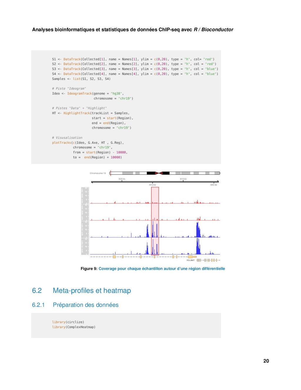
20. Analyses bioinformatiques et statistiques de données ChIP-seq avec R / Bioconductor S1 <- DataTrack(Collected[1], name = Names[1], ylim = c(0,20), type = "h", col= "red") S2 <- DataTrack(Collected[2], name = Names[2], ylim = c(0,20), type = "h", col = "red") S3 <- DataTrack(Collected[3], name = Names[3], ylim = c(0,20), type = "h", col = "blue") S4 <- DataTrack(Collected[4], name = Names[4], ylim = c(0,20), type = "h", col = "blue") Samples <- list(S1, S2, S3, S4) # Piste "Ideogram" Ideo <- IdeogramTrack(genome = "hg38", chromosome = "chr19") # Pistes "Data" + "Highlight" HT <- HighlightTrack(trackList = Samples, start = start(Region), end = end(Region), chromosome = "chr19") # Visusalisation plotTracks(c(Ideo, G_Axe, HT , G_Reg), chromosome = "chr19", from = start(Region) - 10000, to = end(Region) + 10000) Chromosome 19 605 kb 610 kb 615 kb 620 kb 0 5 10 15 20 ESR1_DMSO_REP1 0 5 10 15 20 ESR1_DMSO_REP2 0 5 10 15 20 ESR1_ES_REP1 0 5 10 15 20 ESR1_ES_REP2 POLRMT Figure 9: Coverage pour chaque échantillon autour d’une région différentielle 6.2 Meta-profiles et heatmap 6.2.1 Préparation des données library(circlize) library(ComplexHeatmap) 20
21. Analyses bioinformatiques et statistiques de données ChIP-seq avec R / Bioconductor # Créer un GRange correpondant aux pics différentiels Target_GR <- GRanges(seqnames = seqnames(Simplified), ranges = IRanges(start = Simplified$best.pos - 1000, end = Simplified$best.pos + 1000), strand = "*") # Créer une GRangeList (chaque slot correpondant à un pic +/- 1000 bp, # et contenant un GRange listant la position de 250 fenêtres au sein du pic) Target_GR_Split <- tile(Target_GR, n = 250) # Transformer la GRangeList en GRange Target_GR_Split <- unlist(Target_GR_Split) # Etablir la matrice de comptage # ncol = nombre d'échantillons, # nrow = nombre de pics * 250 Count_Target_GR <- summarizeOverlaps(Target_GR_Split, Bam_Path, yieldSize = 100000, ignore.strand = TRUE, inter.feature = FALSE) # Convertir l'objet SummerizedExperiment en matrice Count_Target_GR <- assay(Count_Target_GR) # Normaliser par le RPM Count_Target_GR <- cpm(Count_Target_GR, log = T) # Générer une matrice indépendante pour chaque échantillon # ncol = 250 # nrow = nombre de pics Count_Target_GR_List <- list() Count_Target_GR_List[[1]] <- t(matrix(Count_Target_GR[,1], nrow = 250)) Count_Target_GR_List[[2]] <- t(matrix(Count_Target_GR[,2], nrow = 250)) Count_Target_GR_List[[3]] <- t(matrix(Count_Target_GR[,3], nrow = 250)) Count_Target_GR_List[[4]] <- t(matrix(Count_Target_GR[,4], nrow = 250)) # Procéder à un lissage par moyenne glissante library(zoo) Smooth_fun <- function(x) { Smooth <- t(rollapply(t(x) , width = 20, by = 1, FUN = mean, partial = TRUE)) return(Smooth) } Count_Smooth <- lapply(Count_Target_GR_List, Smooth_fun) 6.2.2 Meta-profile # Créer deux listes distinctes pour stocker les matrices # de comptage pour les pics "UP" et "DOWN" Up <- which(Simplified$best.logFC > 0) Up_List <- list(Count_Smooth[[1]][Up,], Count_Smooth[[2]][Up,], Count_Smooth[[3]][Up,], 21
22. Analyses bioinformatiques et statistiques de données ChIP-seq avec R / Bioconductor Count_Smooth[[4]][Up,]) Up_List <- lapply(Up_List, colMeans) Down <- which(Simplified$best.logFC < 0) Down_List <- list(Count_Smooth[[1]][Down,], Count_Smooth[[2]][Down,], Count_Smooth[[3]][Down,], Count_Smooth[[4]][Down,]) Down_List <- lapply(Down_List, colMeans) # Créer un data.frame au format adapté à ggplot Meta <- data.frame(Count = c(unlist(Up_List), unlist(Down_List)), Type = c(rep("UP", length(c(unlist(Up_List)))), rep("DOWN", length(c(unlist(Down_List))))), Sample = rep(rep(gsub("_REP[12]", "", Names), each = 250), 2), Position = rep(seq(-125,124), 8)) # Générer les méta-profils ggplot(Meta, aes(y = Count, x = Position, color = Sample)) + geom_smooth(aes(group = Sample)) + facet_grid(~ Type) + xlab("Position relative to the middle of the peak") + ylab("Average normalized read density") DOWN UP 2 3 4 −100 −50 0 50 100 −100 −50 0 50 100 Position relative to the middle of the peak Average normalized read density Sample ESR1_DMSO ESR1_ES Figure 10: Metaprofiles des coverages +/- 1000 bp autour du centre des pics 6.2.3 Heatmap # Définir l'ordre des pics selon le logFC Order <- order(Simplified$best.logFC) # Definir le schema de couleur Color <- colorRampPalette(c("red", "yellow"))(100) 22
23. Analyses bioinformatiques et statistiques de données ChIP-seq avec R / Bioconductor # Définir l'annotation des lignes des heatmaps Split_1 <- c(rep("DOWN", length(which(Simplified$best.logFC[(order(Simplified$best.logFC))]<0))), rep("UP", length(which(Simplified$best.logFC[(order(Simplified$best.logFC))]>0)))) Split_2 <- rowAnnotation(df = data.frame(Change = Split_1), col = list(Change = c("DOWN" = "firebrick1", "UP" = "chartreuse3"), width = unit(.3, "cm"))) # Créer une fonction basée sur Heatmap # et personnalisant les paramètres Heatmap_Custom <- function(x, y) { Heatmap(x, cluster_rows = FALSE, cluster_columns = FALSE, col = Color, column_title = y, split = Split_1, gap = unit(3, "mm"), combined_name_fun = NULL, show_heatmap_legend = FALSE) } # Générer 4 heatmaps Heatmap_Cell <- Split_2 + Heatmap_Custom(Count_Smooth[[1]][Order,], "DMSO") + Heatmap_Custom(Count_Smooth[[2]][Order,], "DMSO") + Heatmap_Custom(Count_Smooth[[3]][Order,], "ES") + Heatmap_Custom(Count_Smooth[[4]][Order,], "ES") # Dessiner les heatmaps côte-à-côte draw(Heatmap_Cell) DMSO DMSO ES ES Change DOWN UP Figure 11: Heatmap des coverages +/- 1000 bp autour du centre des pics ordonnées par FC 23
24. Analyses bioinformatiques et statistiques de données ChIP-seq avec R / Bioconductor 6.2.4 Test d’enrichissement en motifs library(BSgenome.Hsapiens.UCSC.hg19) library(PWMEnrich) library(PWMEnrich.Hsapiens.background) data("PWMLogn.hg19.MotifDb.Hsap") # Récupérer un fichier chain pour convertir # les coordonnées hg38 vers hg19 Chain <- "http://hgdownload.cse.ucsc.edu/goldenpath/hg38/liftOver/hg38ToHg19.over.chain.gz" download.file(Chain, destfile = "hg38ToHg19.over.chain.gz") gunzip("hg38ToHg19.over.chain.gz", "hg38ToHg19.over.chain", overwrite = T) Chain <- import.chain("hg38ToHg19.over.chain") # Définir les régions d'intérêt Target <- Simplified[which(Simplified$best.logFC > 2)] Target <- GRanges(seqnames = seqnames(Target), IRanges(Target$best.pos - 15, Target$best.pos + 15)) # Procéder à la conversion de coordonnées seqlevels(Target) <- "chr19" seqlengths(Target) <- c(59128983) Target_HG19 <- unlist(liftOver(Target, chain = Chain)) # Récupérer les séquences génomiques # correspondant aux pics sélectionnés Cluster_1_Cell_Seq <- BSgenome::getSeq(BSgenome.Hsapiens.UCSC.hg19, GRanges(Target_HG19)) # Procéder à l'analyse d'enrichissement Motif_Cluster_1_Cell <- motifEnrichment(Cluster_1_Cell_Seq, PWMLogn.hg19.MotifDb.Hsap) # Générer un tableau synthétisant les résultats Motif_Cluster_1_Cell = groupReport(Motif_Cluster_1_Cell) # Afficher les résultats plot(Motif_Cluster_1_Cell[1:10], fontsize=7, id.fontsize=5) 6.2.5 Tests d’enrichissement fonctionnel library(chipenrich) library(plyr) library(rtracklayer) # Préparer les données d'entrée Target_HG19 <- data.frame(Target_HG19)[,c(1:3)] colnames(Target_HG19) <- c("chrom", "start", "end") # Procéder à l'analyse d'enrichissement Results_Cluster_1_Cell <- chipenrich(peaks = Target_HG19[1,], method='chipenrich', fisher_alt = "greater", 24
25. Analyses bioinformatiques et statistiques de données ChIP-seq avec R / Bioconductor Rank Target PWM Motif ID Raw score P−value In top motifs 1 FGF19 FGF19 2.68 0.0000000000000000000822 20 % 2 TAGLN2 TAGLN2 3.1 0.000000000000000000117 18 % 3 CELF6 BRUNOL6 1.86 0.00000000000000000551 21 % 4 SMPX SMPX 5.090.0000000000000000057 18 % 5 TCF3 M3155_1.02 2.090.0000000000000000119 18 % 6 NAP1L1 NAP1L1 3.340.0000000000000000138 20 % 7 HLCS HLCS 2.310.0000000000000000548 18 % 8 CREB1 M3090_1.02 2.120.0000000000000000775 17 % 9 TIMM8A TIMM8A 1.820.0000000000000000807 18 % 10 GRHPR GRHPR 3.640.00000000000000022715 % Figure 12: Logos et scores des 10 motifs les plus enrichis dans les régions UP genesets = c("reactome"), out_path = getwd(), locusdef = "10kb", max_geneset_size = 10, genome = "hg19", n_cores = 1) # Préparer les résultats pour sortie Results_Cluster_1_Cell_ALL <- arrange(Results_Cluster_1_Cell$results, Geneset.Type, FDR) Results_Cluster_1_Cell <- Results_Cluster_1_Cell_ALL[ which(Results_Cluster_1_Cell_ALL$FDR < .2),c(2,3,4,5,9,10)] Results_Cluster_1_Cell 25