x.ordinal compare y.ordinal data RGB = Red | Green | Blue deriving(Eq,Ord,Show) enum RGB : case Red, Green, Blue TestCase (assertEqual "sort integers" [1,2,3,3,4,5] (qsort [5,1,3,2,4,3])) TestCase (assertEqual "sort doubles" [1.1,2.3,3.4,3.4,4.5,5.2] (qsort [5.2,1.1,3.4,2.3,4.5,3.4])) TestCase (assertEqual "sort chars" "abccde" (qsort "acbecd")) TestCase (assertEqual "sort strings" ["abc","efg","uvz"] (qsort ["abc","uvz","efg"]) ) TestCase (assertEqual "sort colours" [Red,Green,Blue] (qsort [Blue,Green,Red])) assert(qsort(List(5,1,2,4,3)) == List(1,2,3,4,5)) assert(qsort(List(5.2,1.1,3.4,2.3,4.5,3.4)) == List(1.1,2.3,3.4,3.4,4.5,5.2)) assert(qsort(List(Blue,Green,Red)) == List(Red,Green,Blue)) assert(qsort("acbecd".toList) == "abccde".toList) assert(qsort(List ("abc","uvz","efg")) == List("abc","efg","uvz")) And here are some Haskell and Scala tests for qsort.
: List[A] = as match case Nil =>](https://files.speakerdeck.com/presentations/f773700df21b4baa868224c11589ee1e/slide_3.jpg)
![given Ordering[RGB] with def compare(x: RGB, y: RGB): Int =](https://files.speakerdeck.com/presentations/f773700df21b4baa868224c11589ee1e/slide_4.jpg)
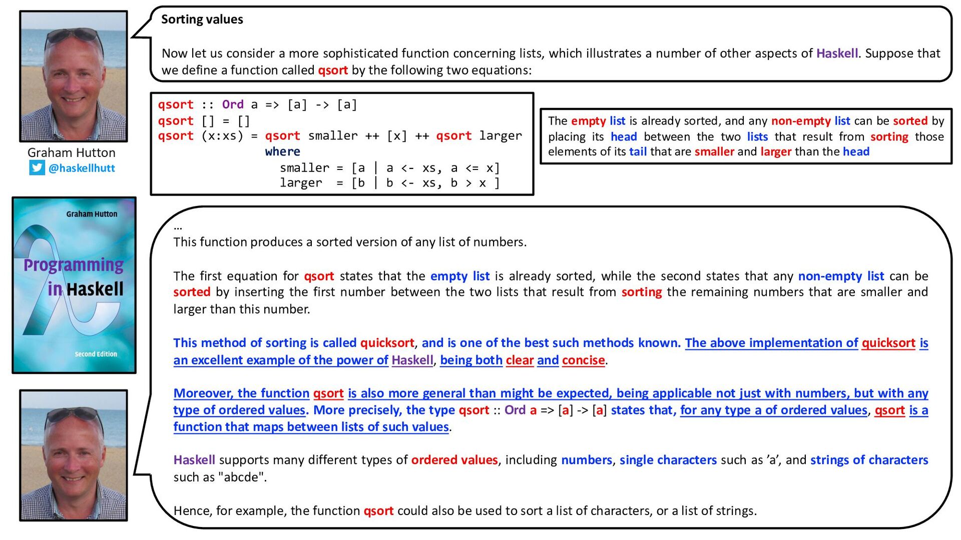
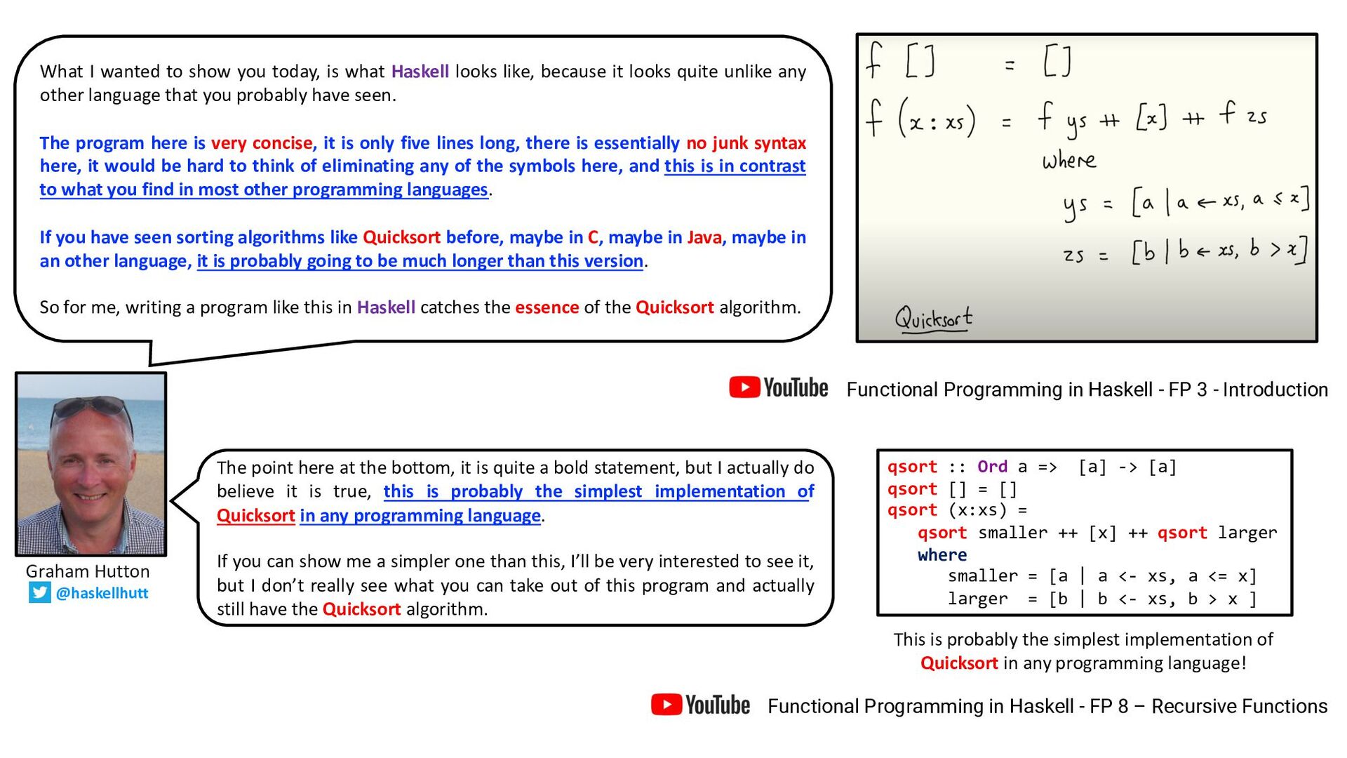
![qsort :: Ord a => [a] -> [a] qsort []](https://files.speakerdeck.com/presentations/f773700df21b4baa868224c11589ee1e/slide_5.jpg)
![qsort :: Ord a => [a] -> [a] qsort []](https://files.speakerdeck.com/presentations/f773700df21b4baa868224c11589ee1e/slide_6.jpg)
![qsort( [], [] ). qsort( [X|XS], Sorted ) :- partition(X,](https://files.speakerdeck.com/presentations/f773700df21b4baa868224c11589ee1e/slide_7.jpg)
: List[A] = xs.headOption.fold(Nil){ x => val smaller](https://files.speakerdeck.com/presentations/f773700df21b4baa868224c11589ee1e/slide_8.jpg)
: List[A] = xs.headOption.fold(Nil){ x => val (smaller,larger)](https://files.speakerdeck.com/presentations/f773700df21b4baa868224c11589ee1e/slide_9.jpg)
![partition p = foldr f ([],[]) where f y (ys,zs)](https://files.speakerdeck.com/presentations/f773700df21b4baa868224c11589ee1e/slide_19.jpg)