本投影片介紹 Raspberry Pi Camera + Python + OpenCV,配合實體課程 8 小時(共 16 小時,這是第二天內容),涵蓋以下內容:
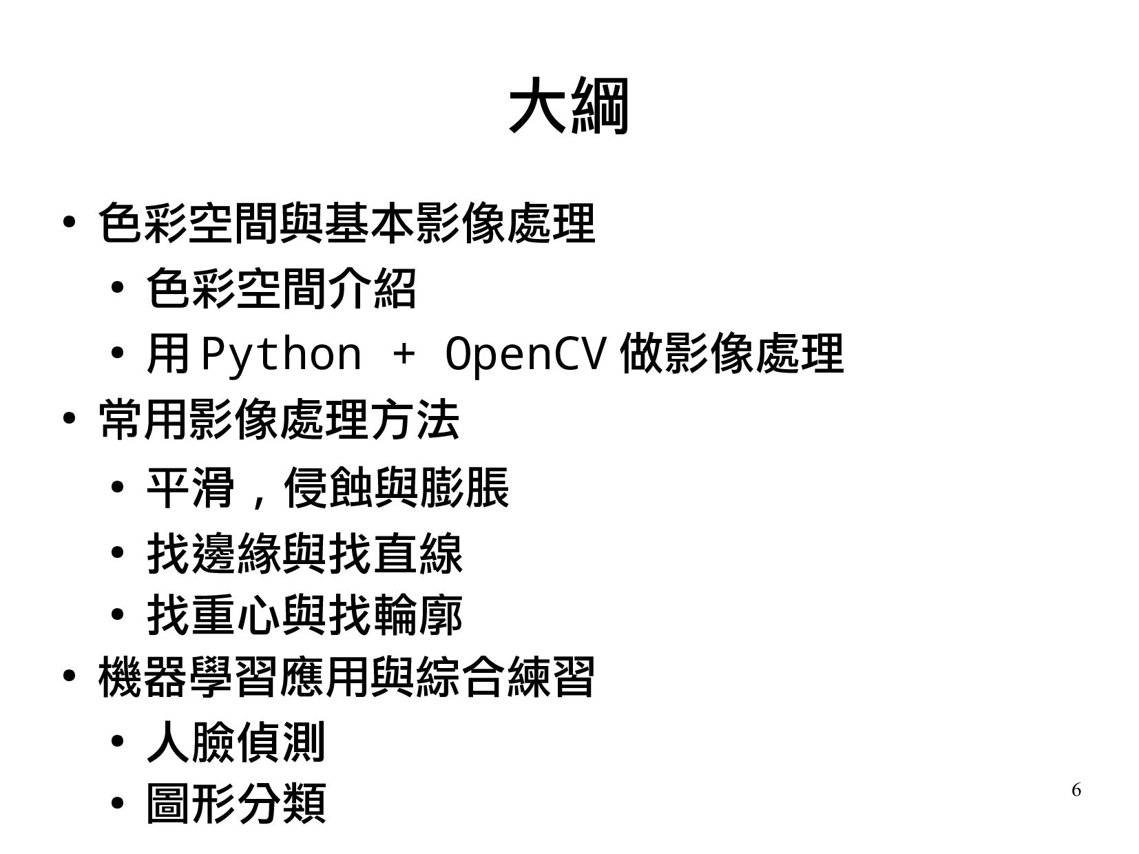
1.色彩空間與基本影像處理(2 小時)
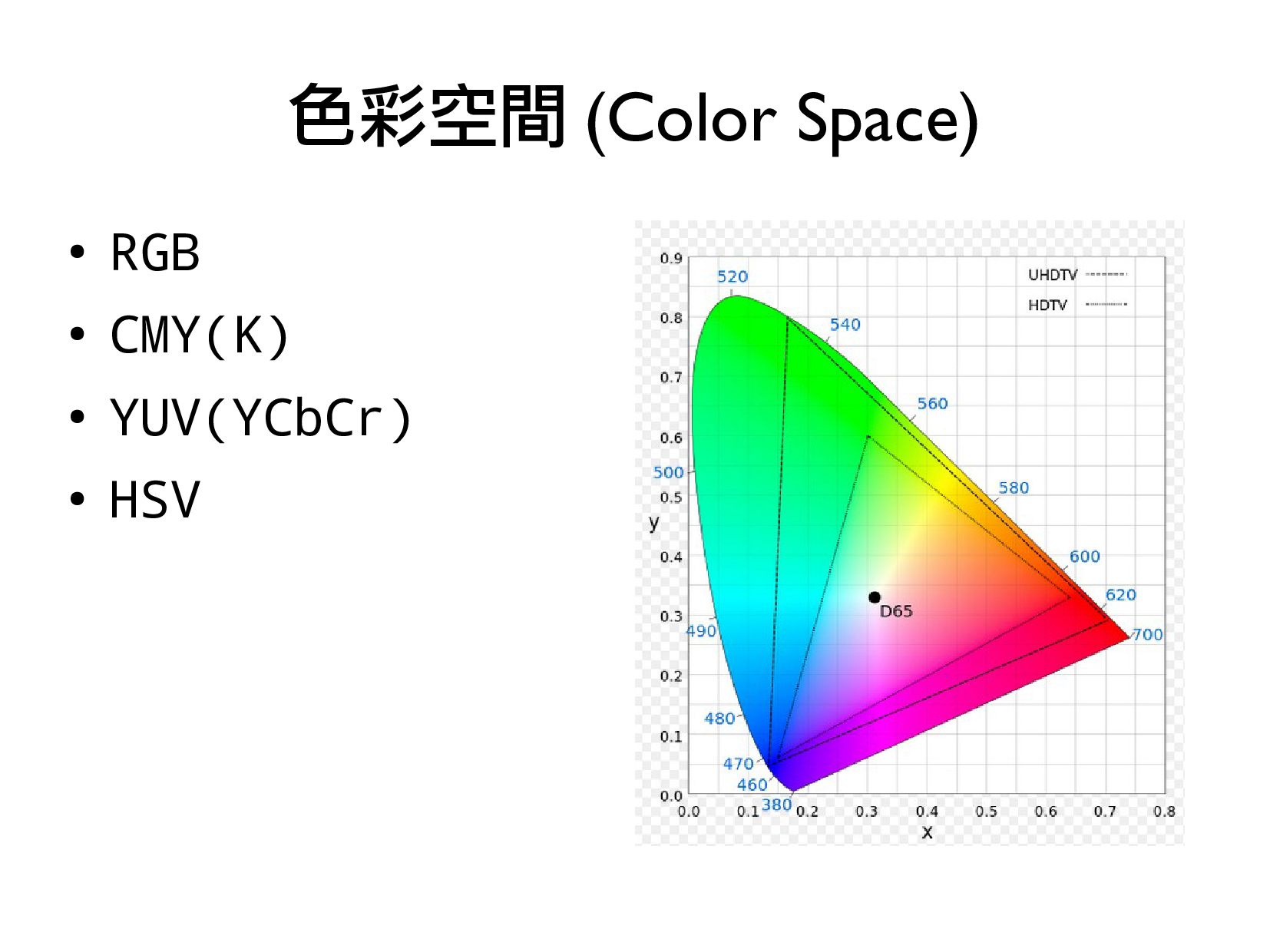
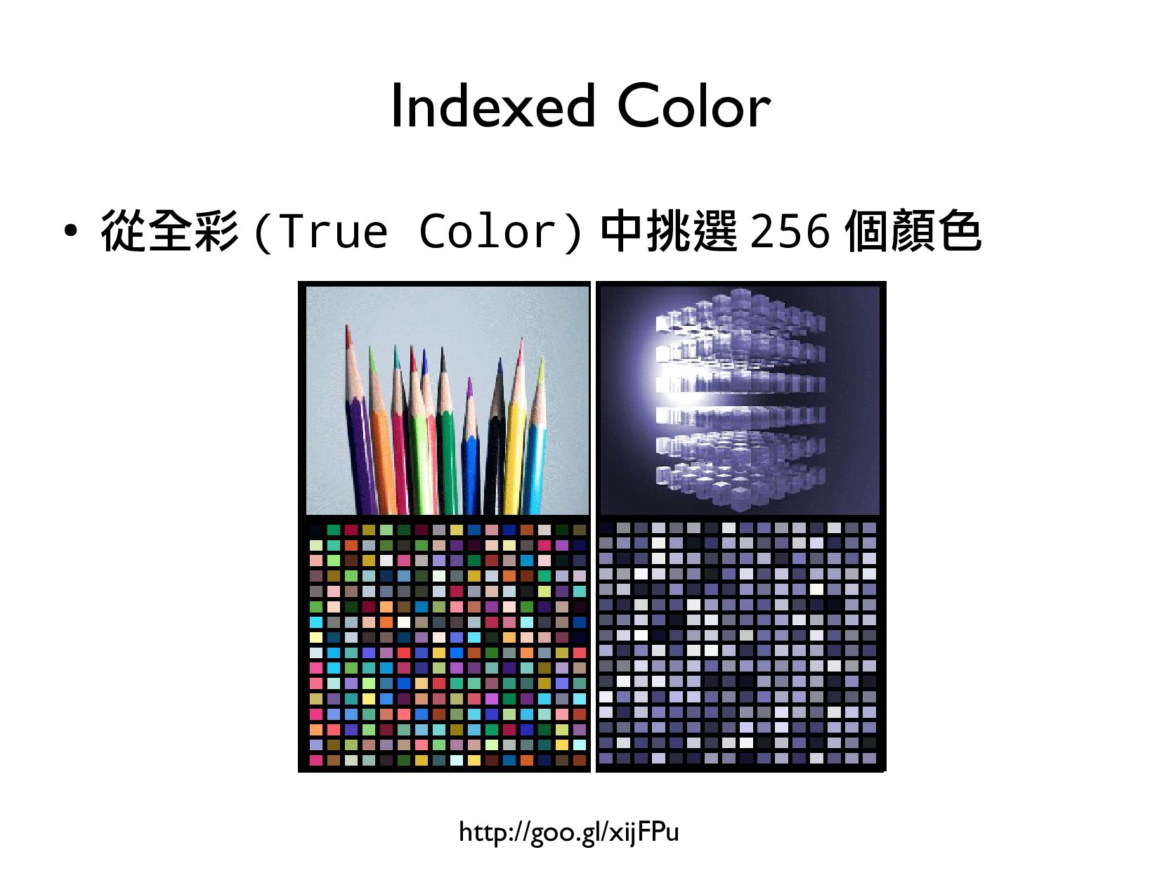
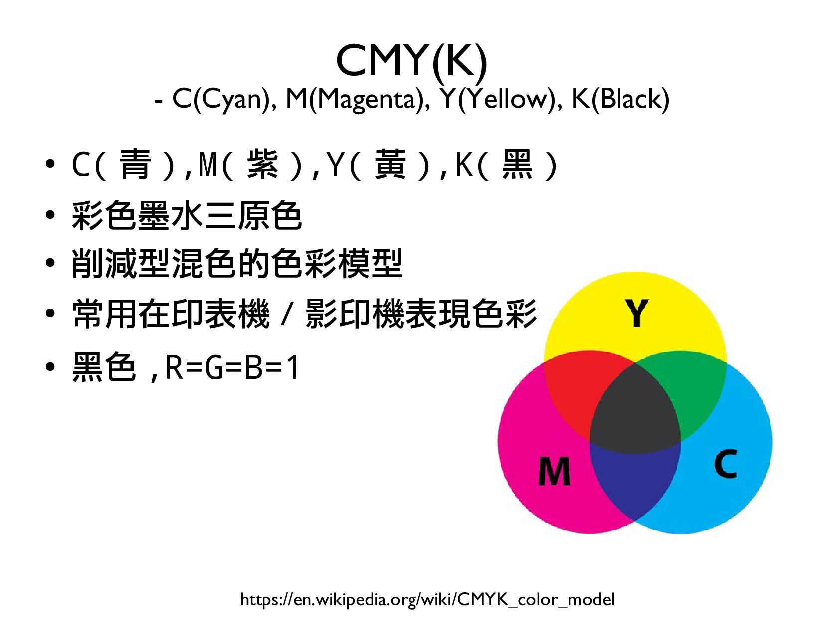
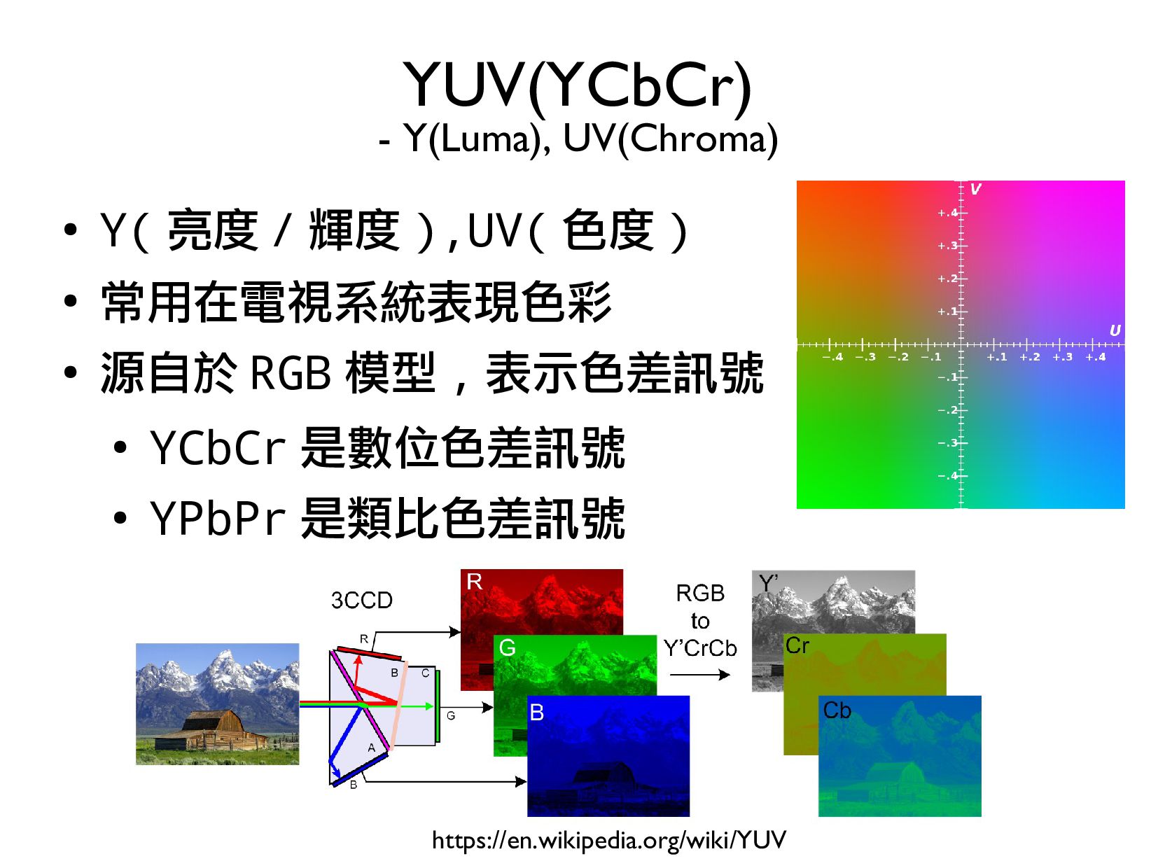
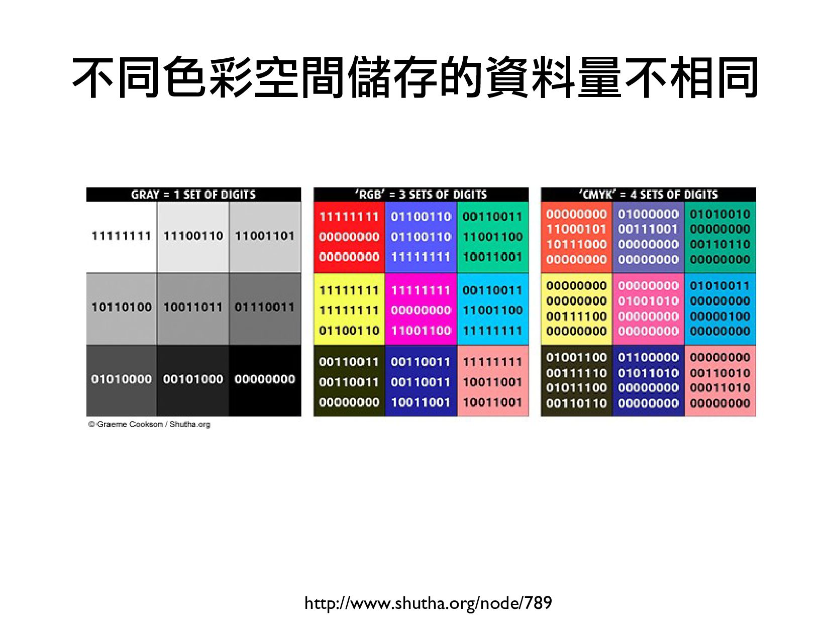
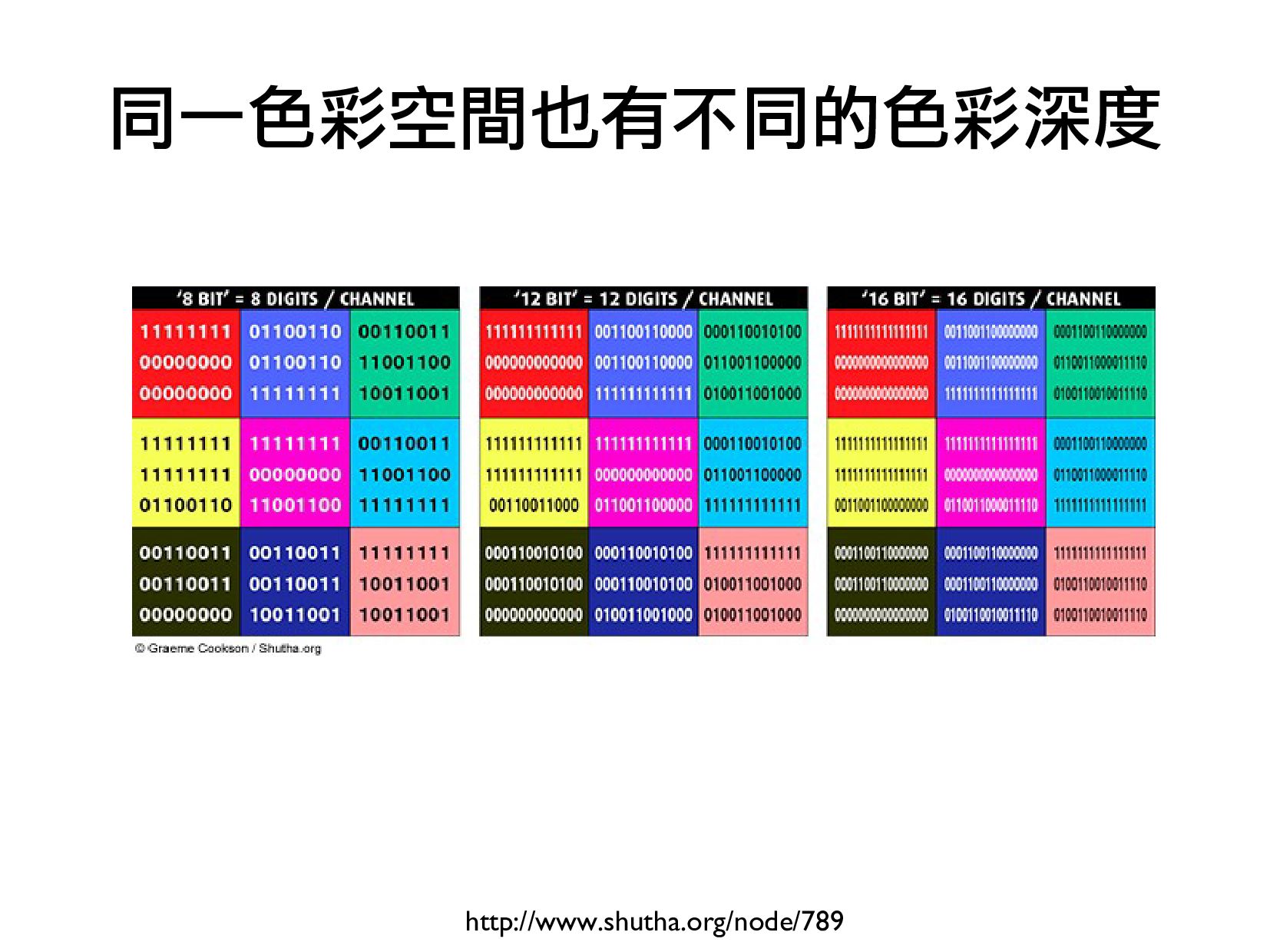
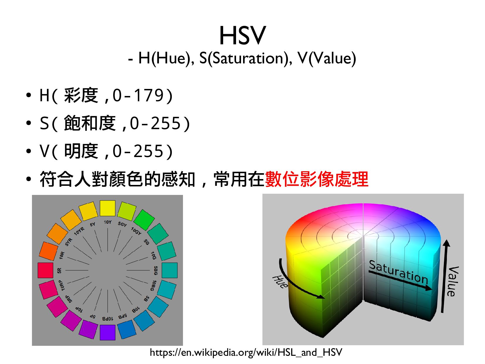
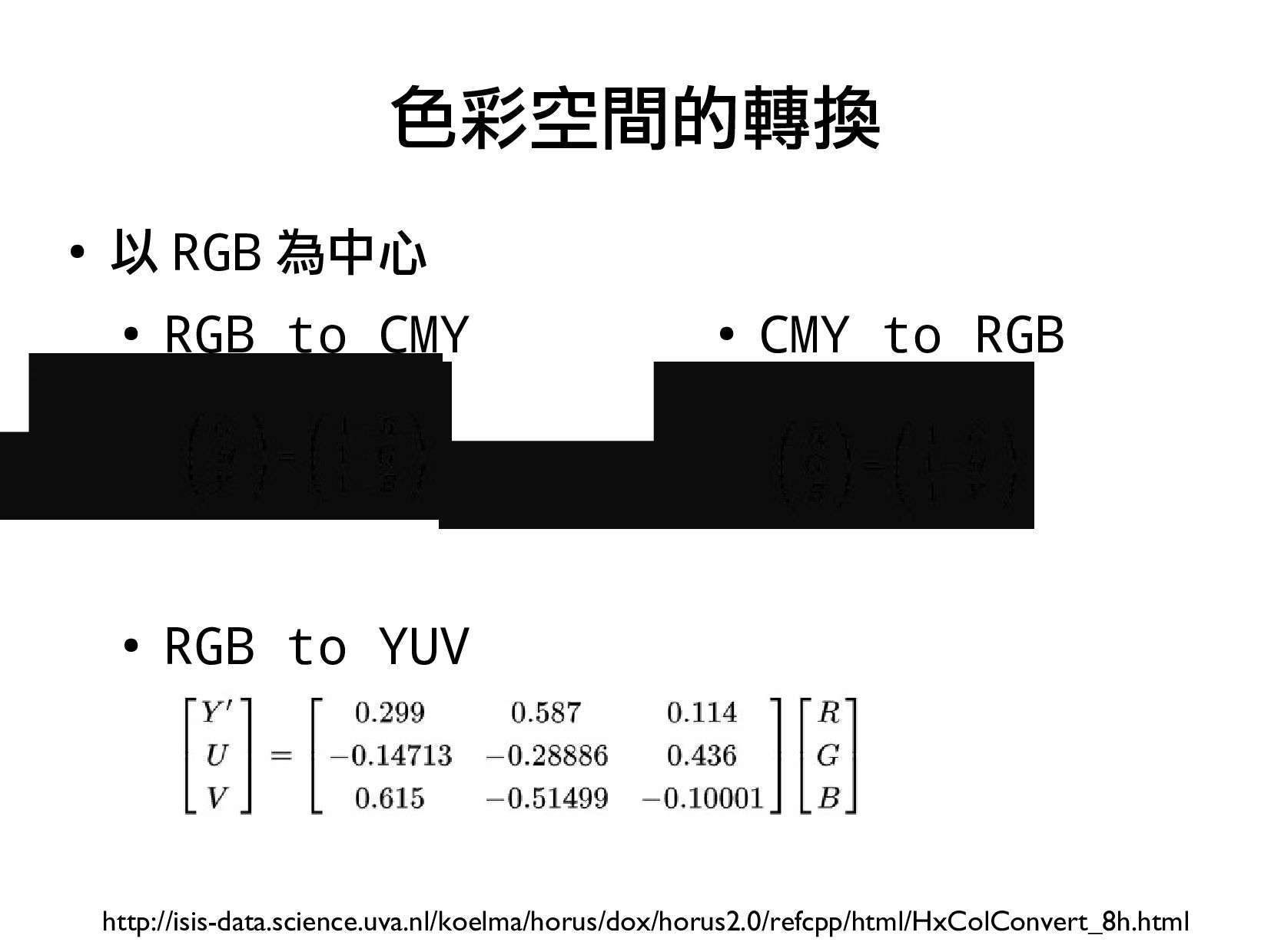
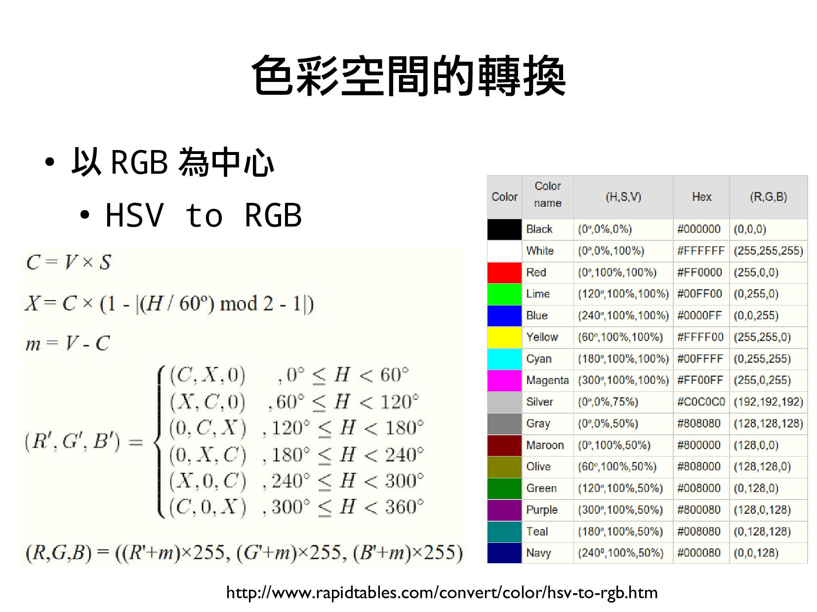
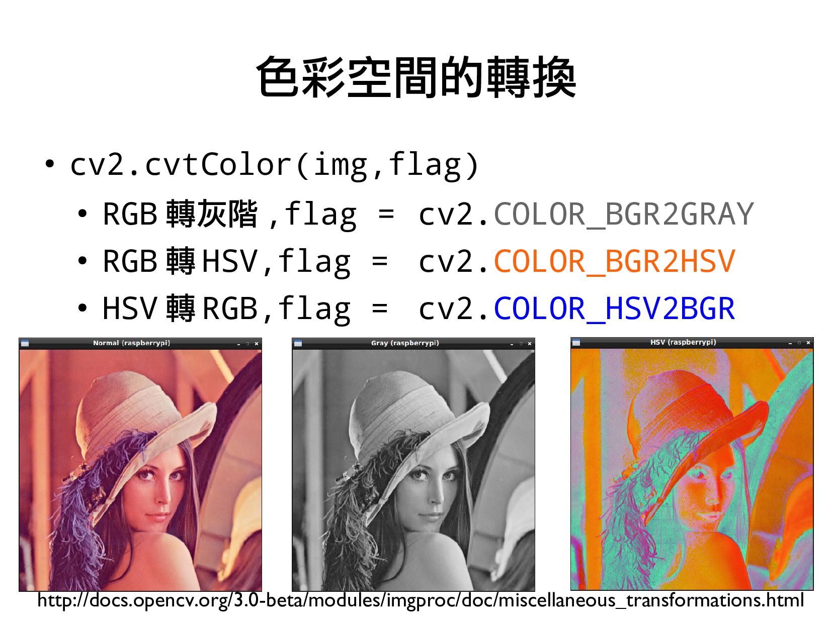
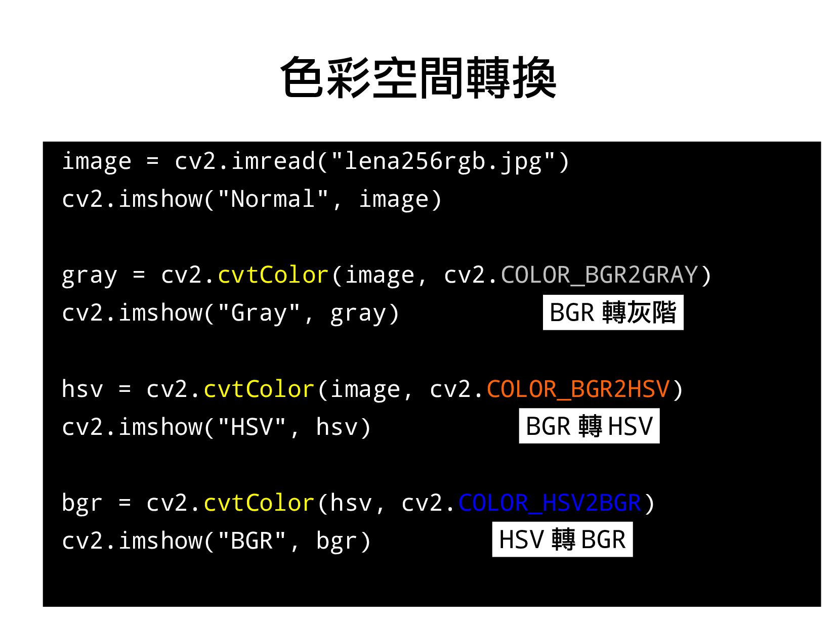
- 色彩空間介紹
- 用 Python + OpenCV 做影像處理
2.常用影像處理方法(3 小時)
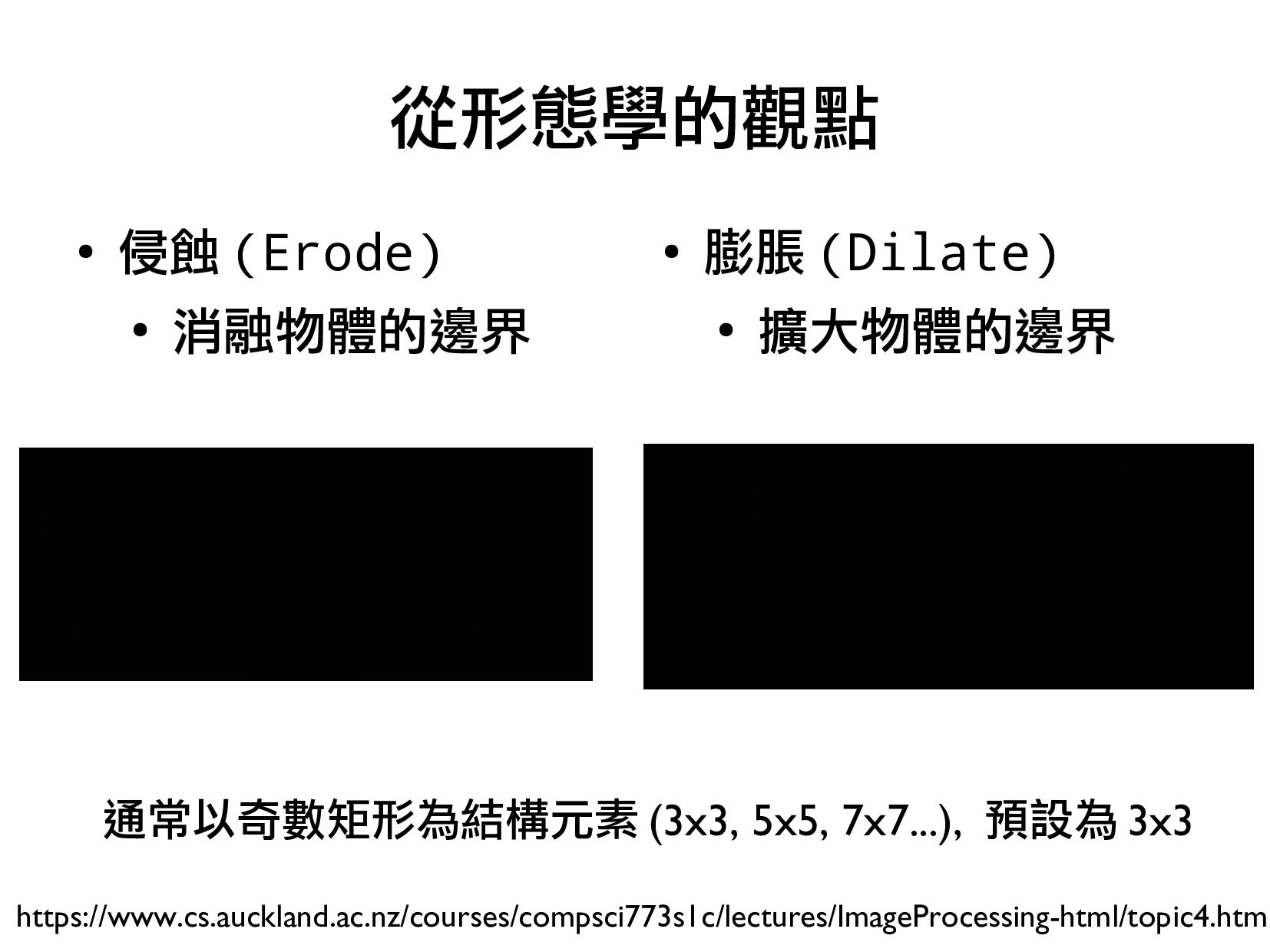
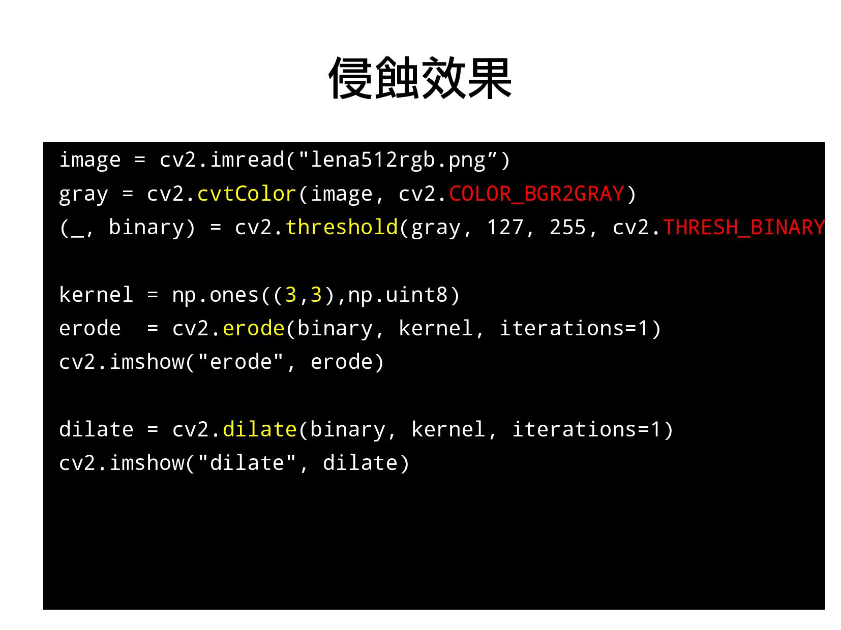
- 平滑,侵蝕與膨脹
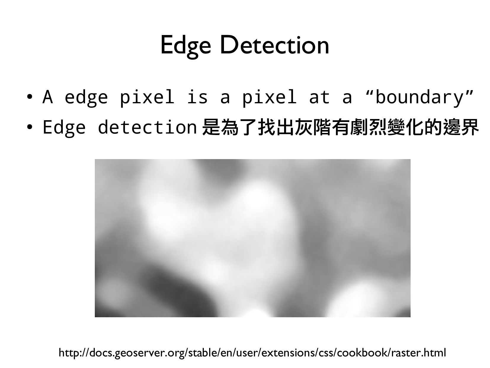
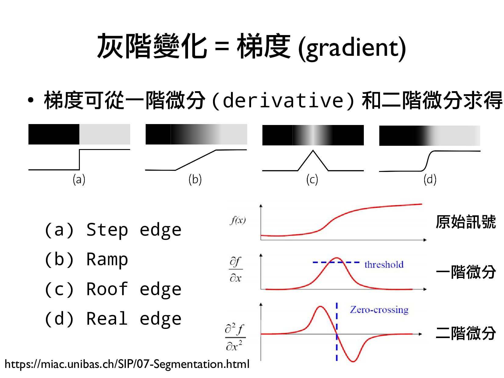
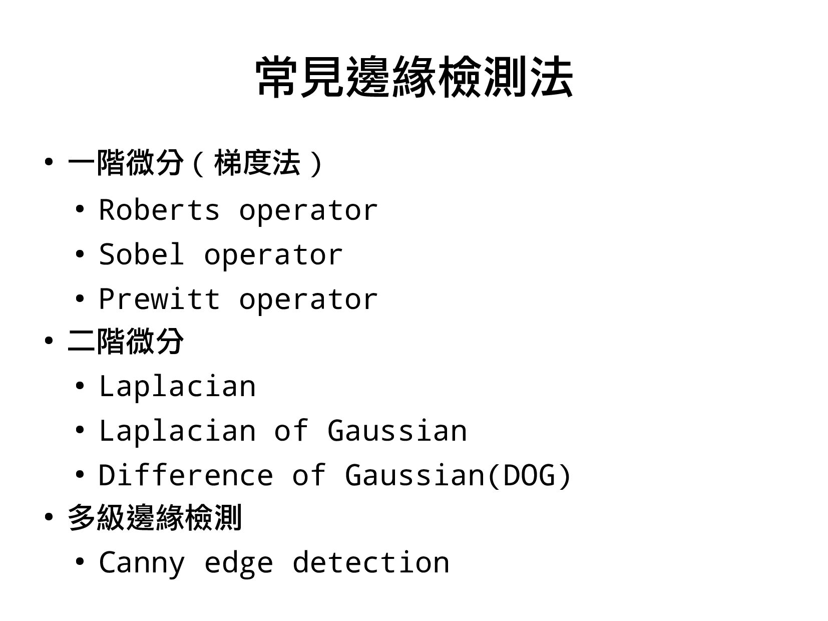
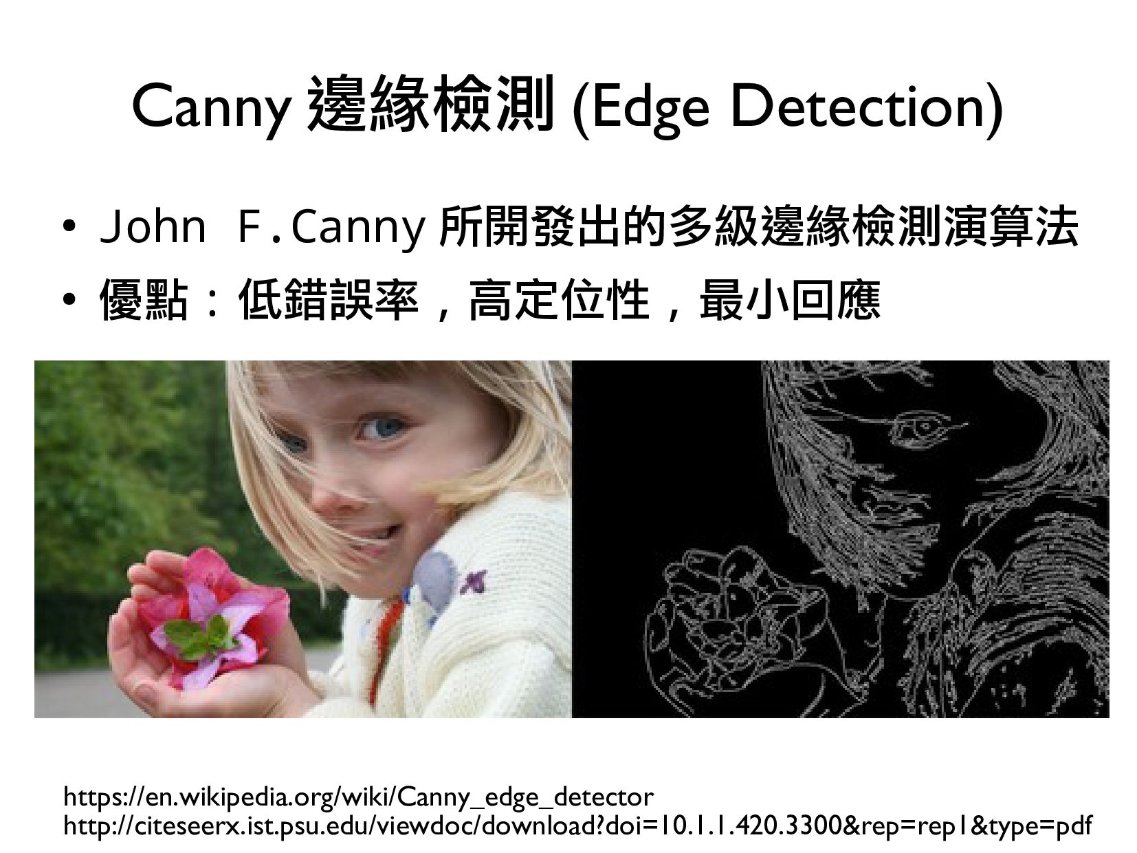
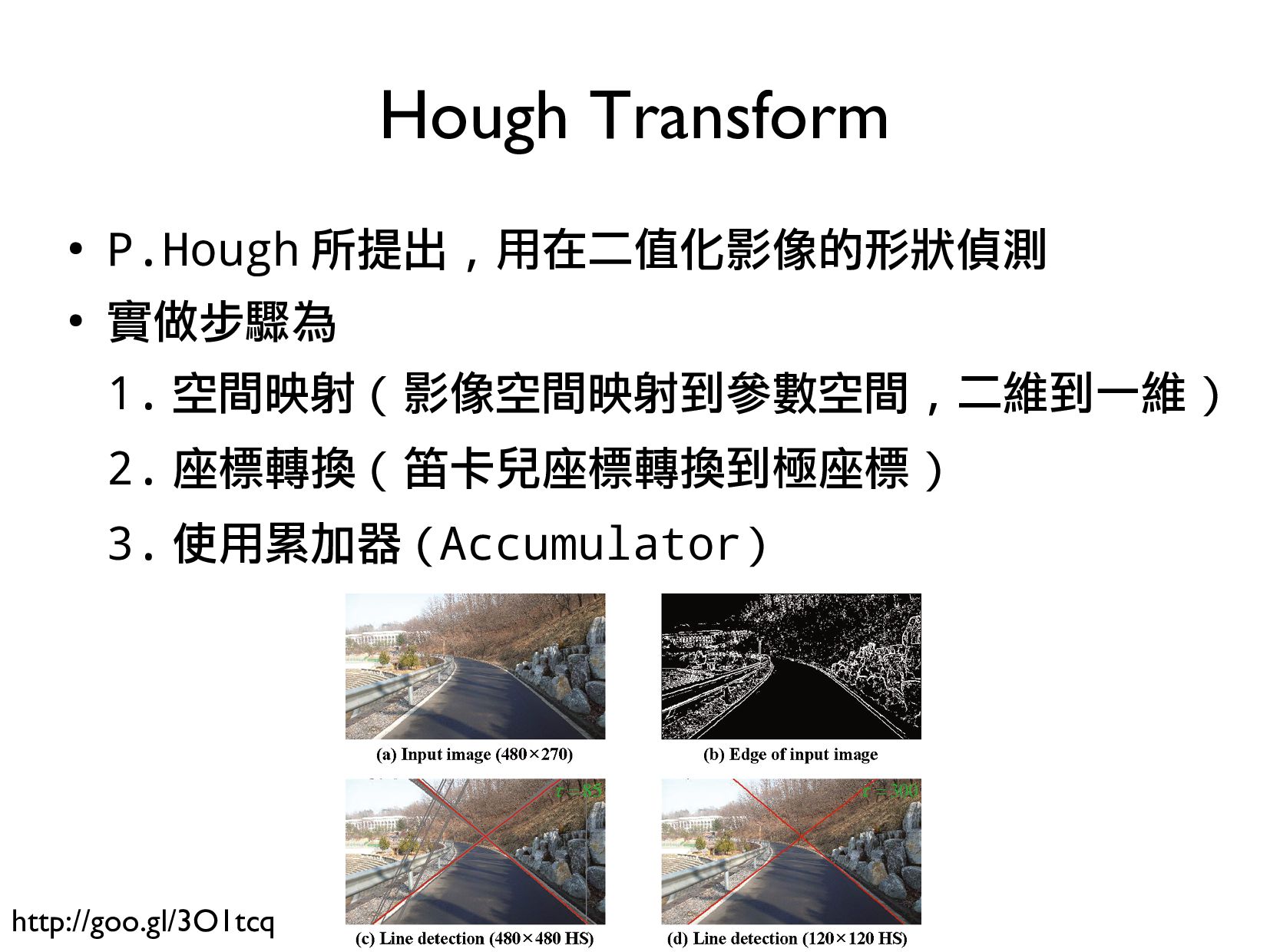
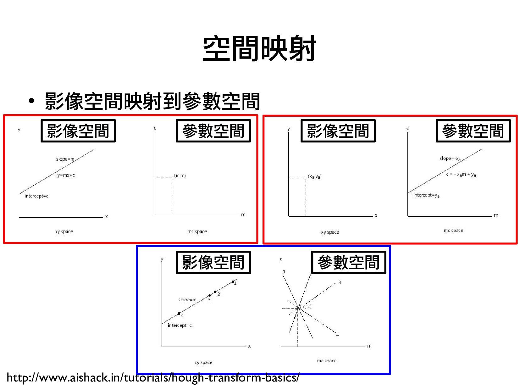
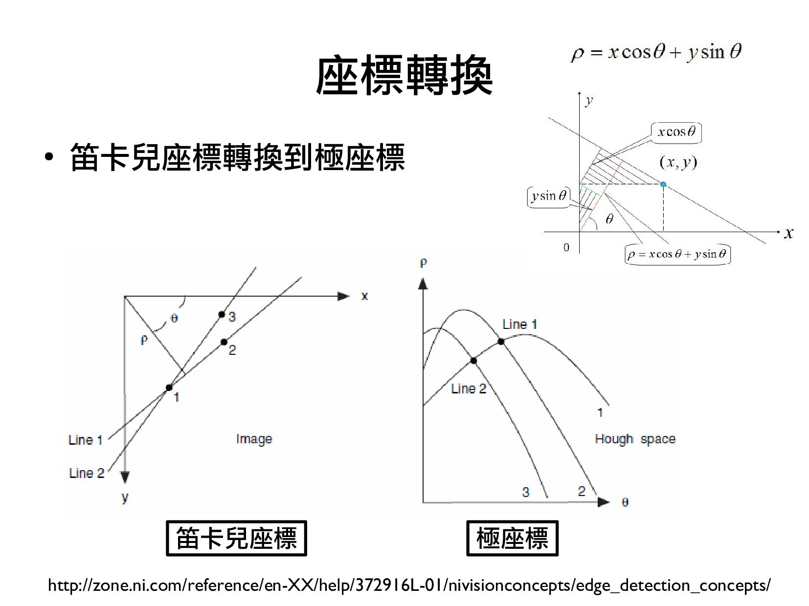
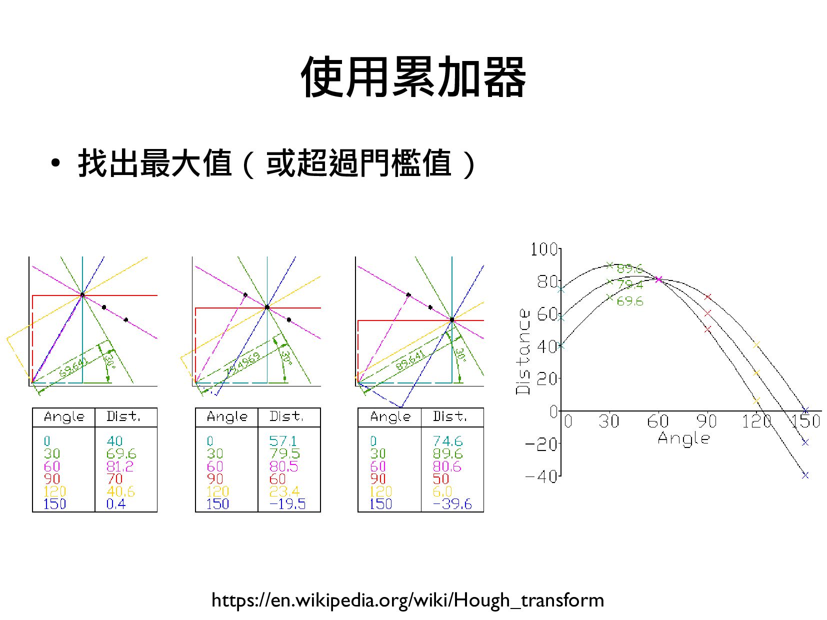
- 找邊緣與找直線
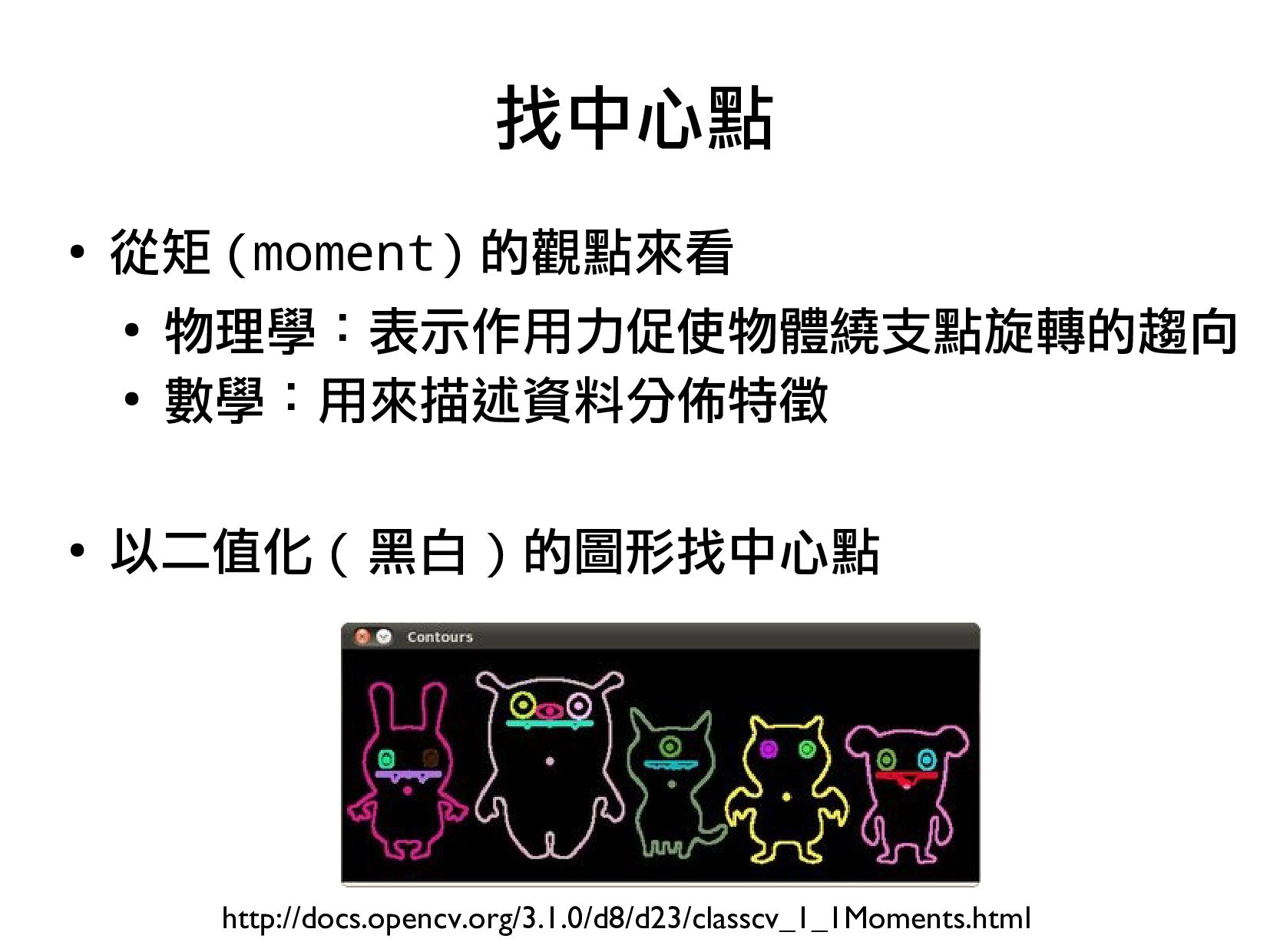
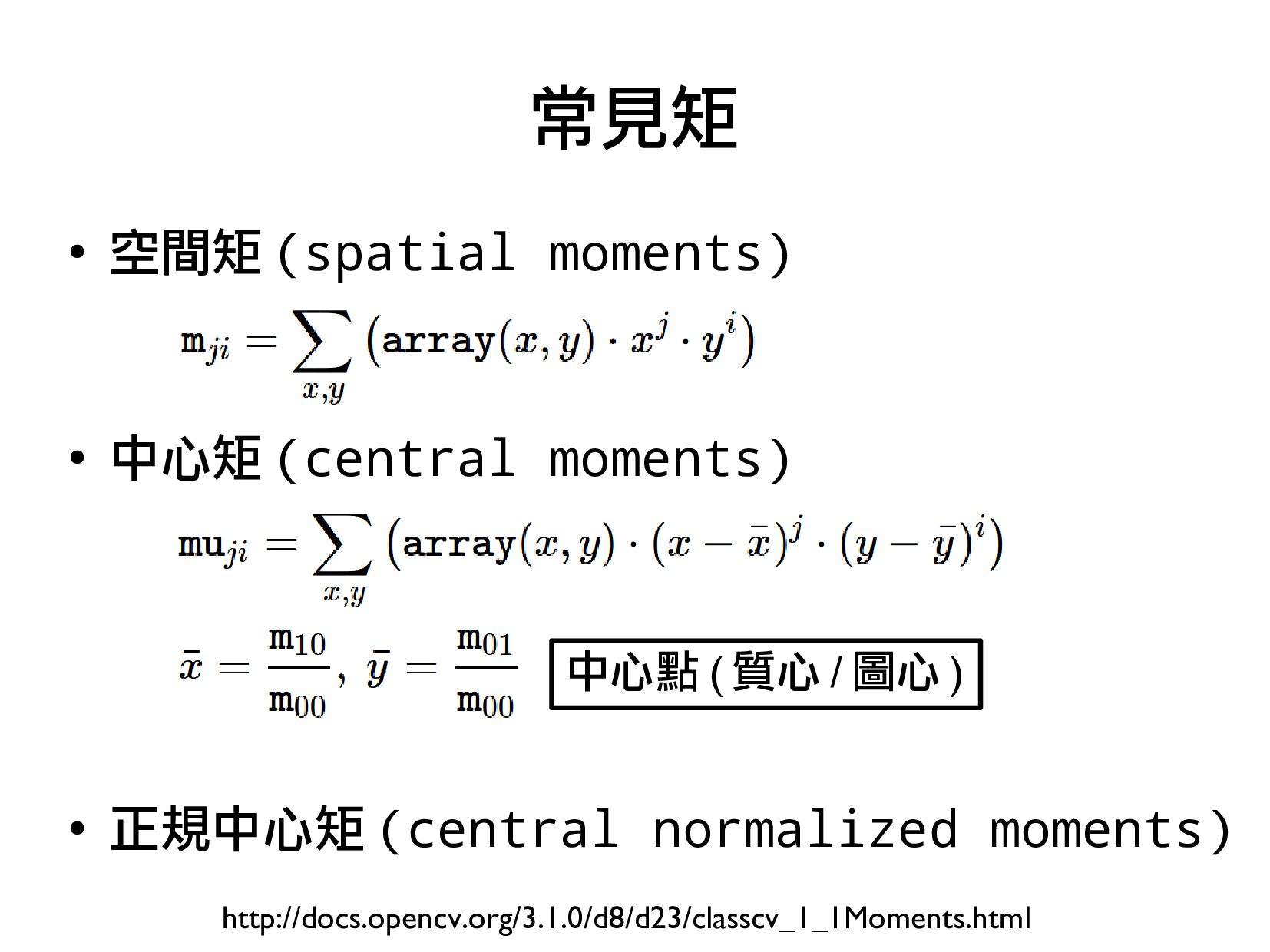
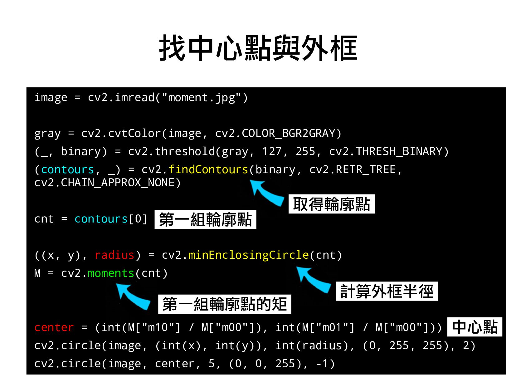
- 找重心與找輪廓
3.機器學習應用與綜合練習(3 小時)
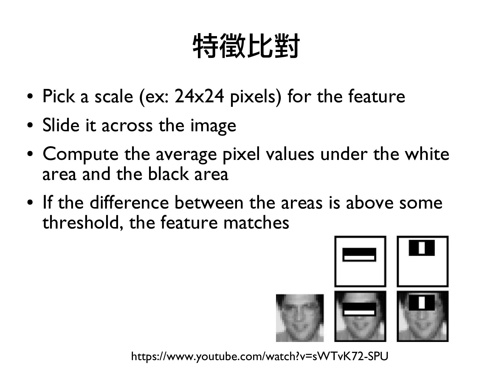
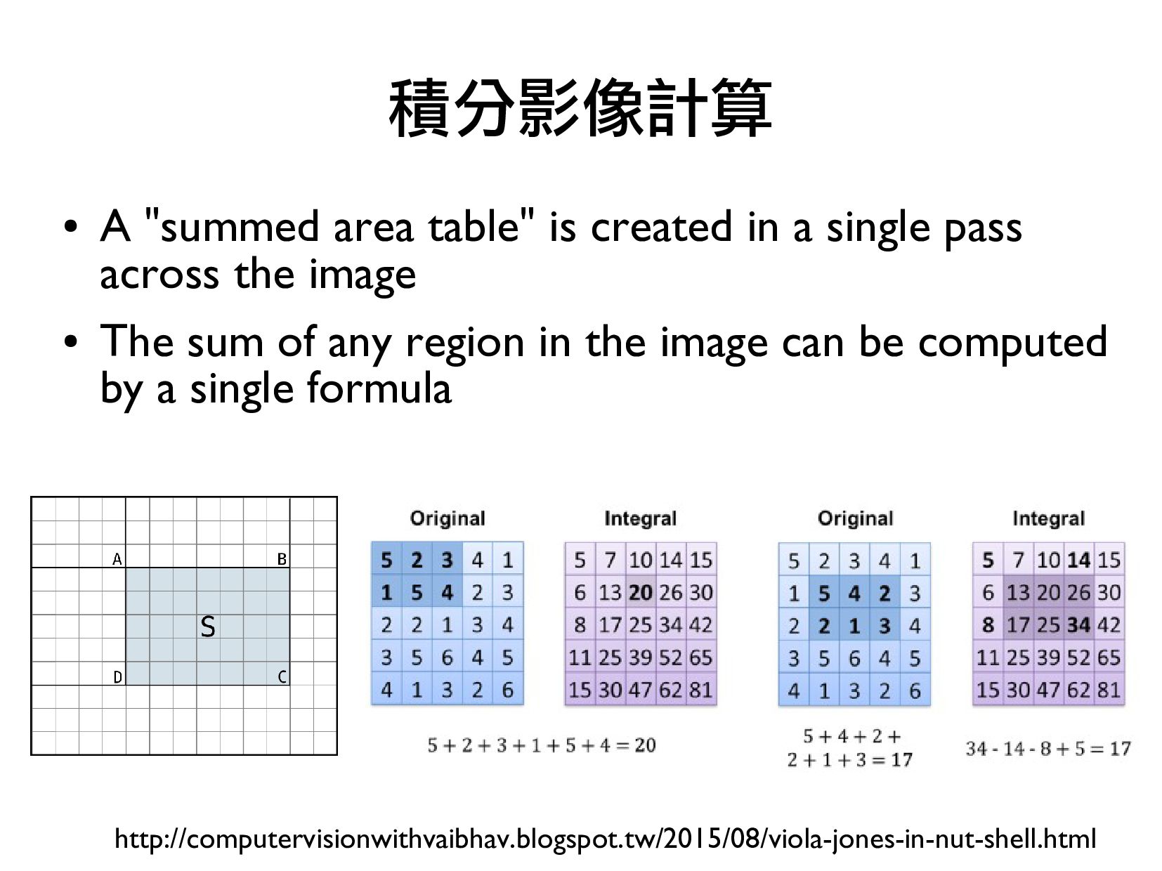
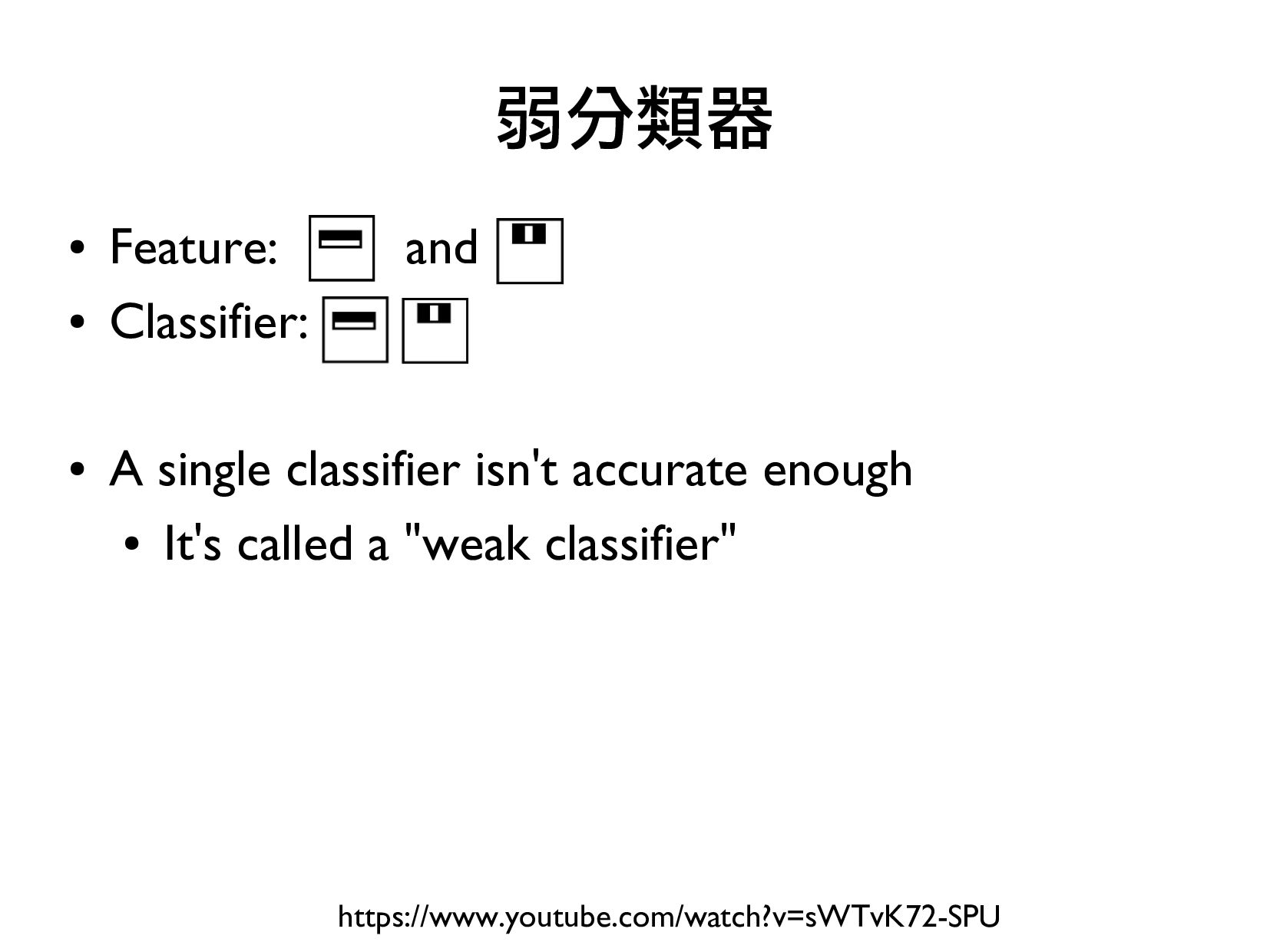
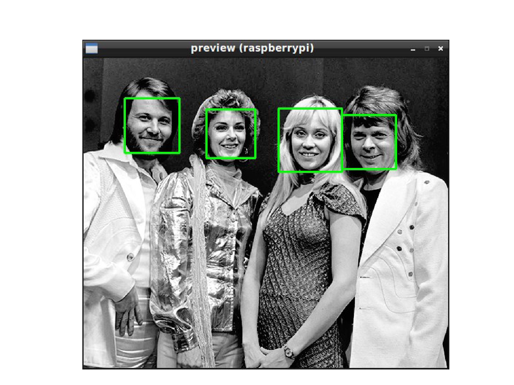
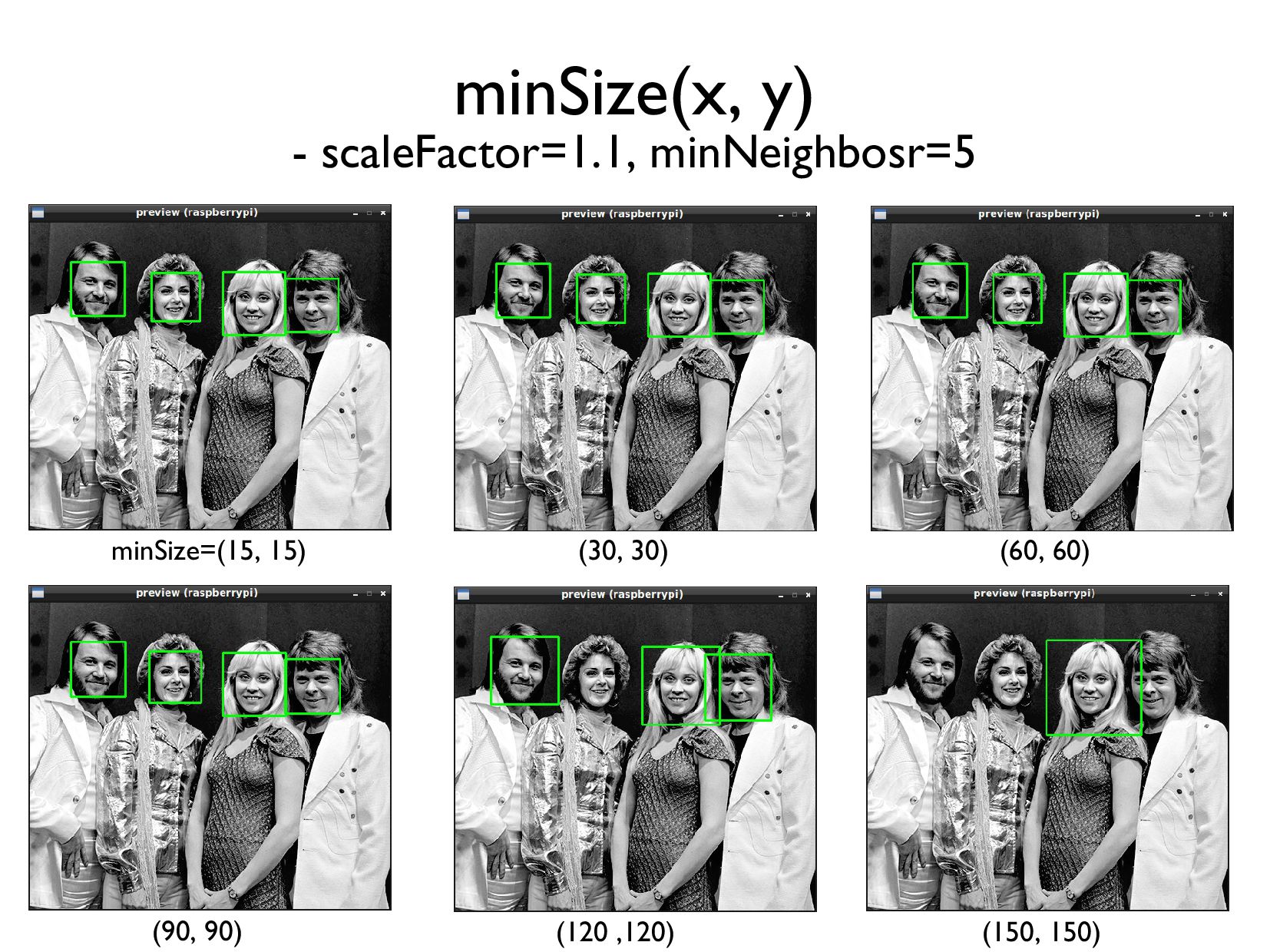
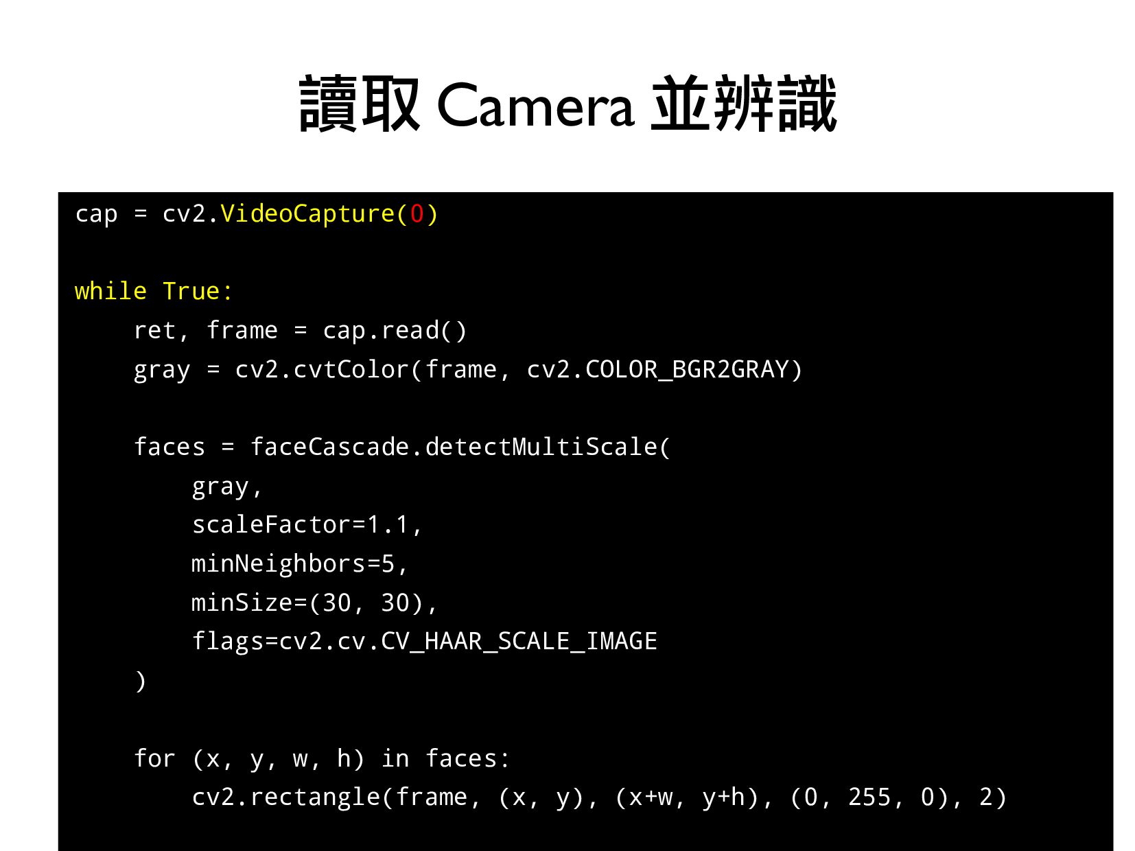
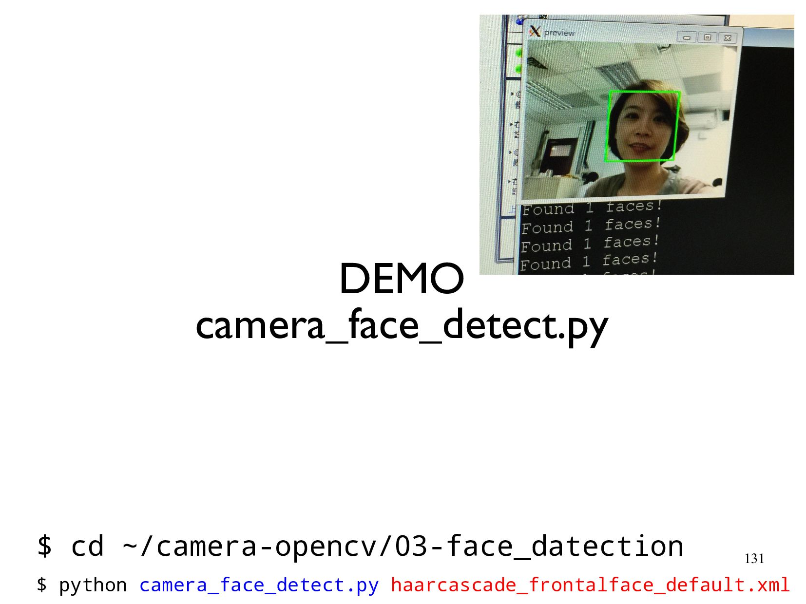
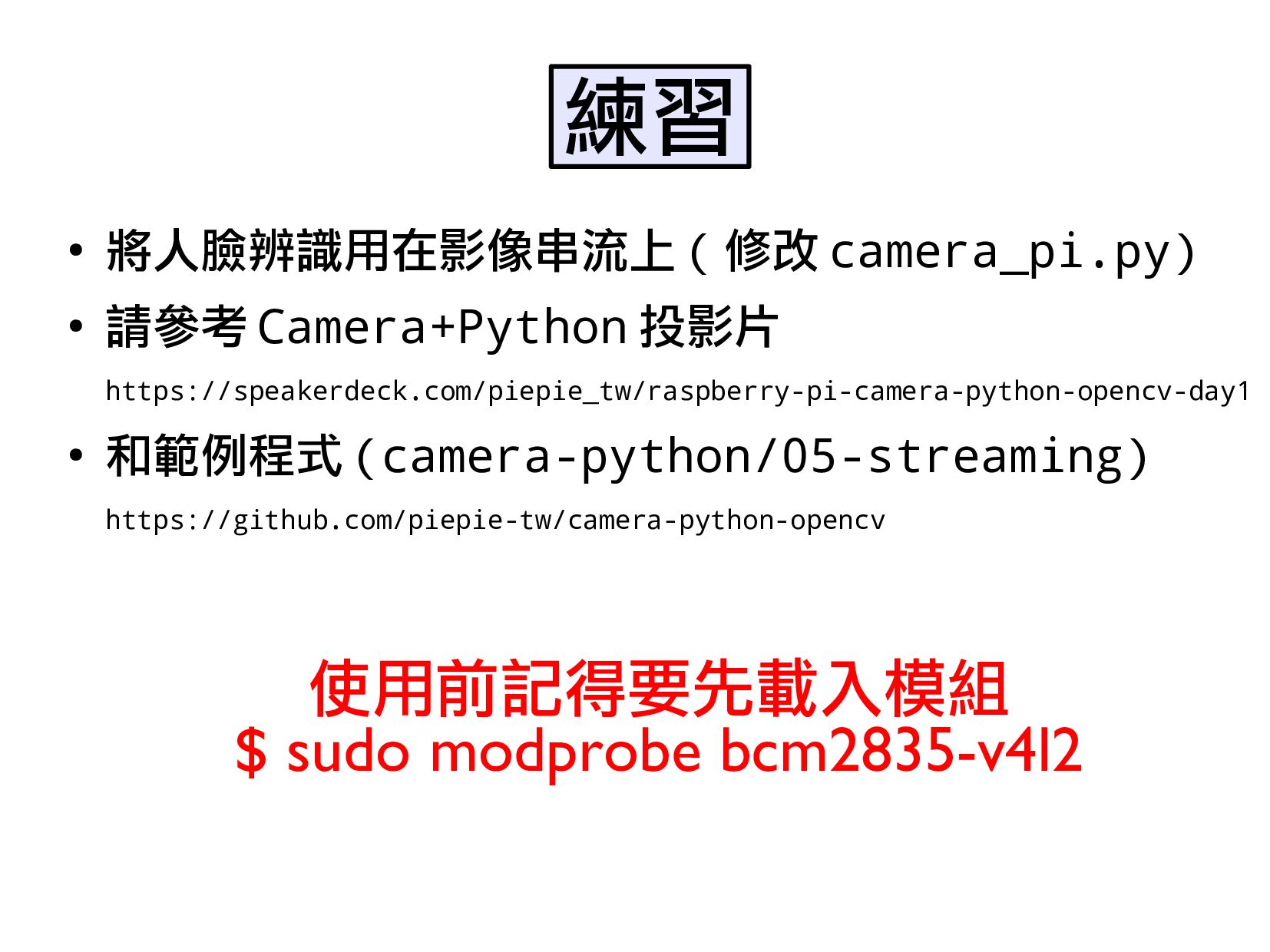
- 人臉偵測
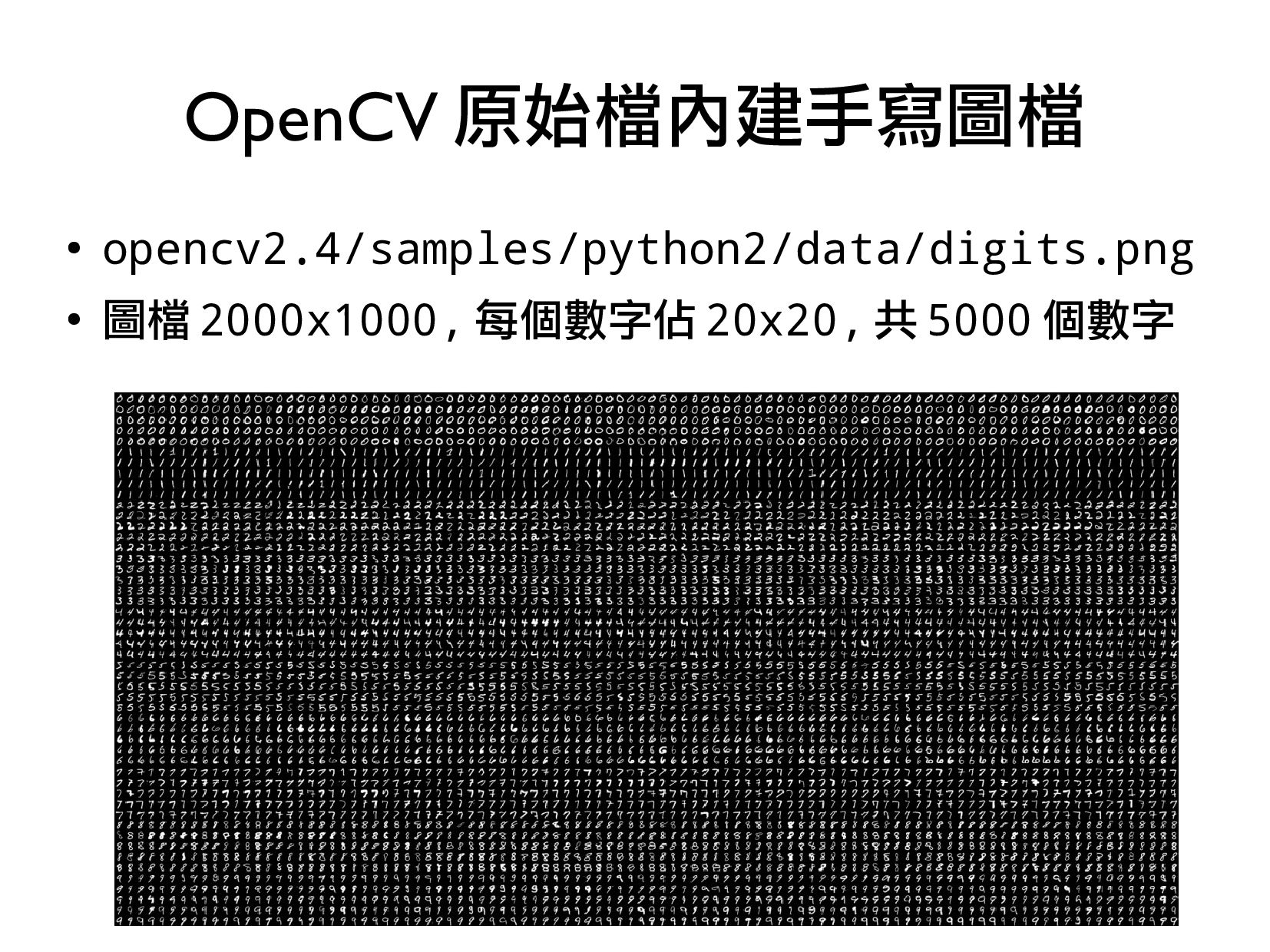
- 圖形分類(手寫辨識)
購買 Pi 3:
https://www.piepie.com.tw/10684/raspberry-pi-3-model-b
購買相機:
https://www.piepie.com.tw/12085/raspberrypi-camera-module-v2
https://www.piepie.com.tw/12056/raspberrypi-noir-camera-module-v2
範例程式:
https://github.com/piepie-tw/camera-python-opencv
Day1 投影片:
https://speakerdeck.com/piepie_tw/raspberry-pi-camera-python-opencv-day1
![Raspberry Pi Camera and OpenCV 台灣樹莓派 <[email protected]> 2017/07/28 @NFU](https://files.speakerdeck.com/presentations/79bbc2dc35484f3c9702a196c6f6cd5a/slide_0.jpg)
![>>> b = np.array(["1", 2]) >>> b.ndim 1 >>> b.shape](https://files.speakerdeck.com/presentations/79bbc2dc35484f3c9702a196c6f6cd5a/slide_12.jpg)
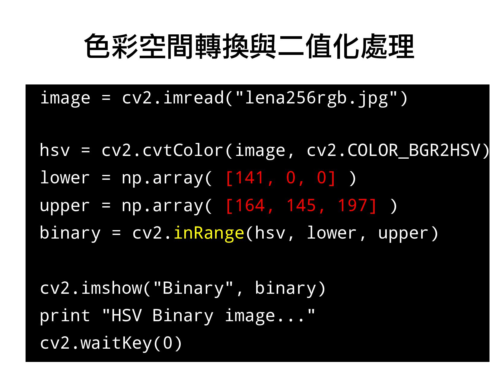
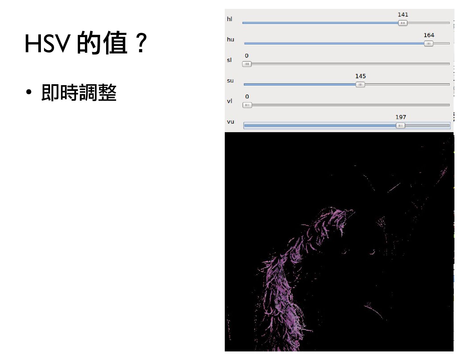
![• cv2.inRange(img,lowerval,upperval) • 範例 : 只取出紫色部份 • lower=np.array([141,0,0]) • upper=np.array([164,145,197])](https://files.speakerdeck.com/presentations/79bbc2dc35484f3c9702a196c6f6cd5a/slide_36.jpg)
![• cv2.erode(src, kernel[, iterations]) • iterations – number of times](https://files.speakerdeck.com/presentations/79bbc2dc35484f3c9702a196c6f6cd5a/slide_73.jpg)
![• cv2.dilate(src, kernel[, iterations]) • iterations – number of times](https://files.speakerdeck.com/presentations/79bbc2dc35484f3c9702a196c6f6cd5a/slide_74.jpg)
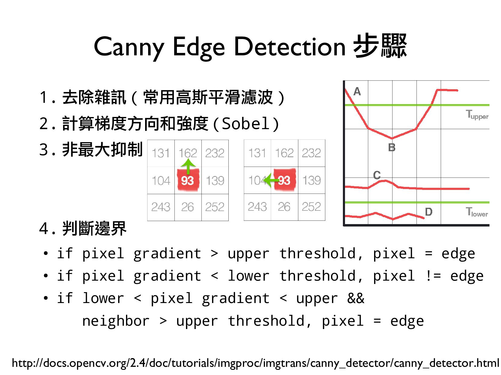
![• cv2.Canny(img,lowerT,upperT,[apertureSize]) • 通常上下門檻值的比例在 2:1 到 3:1 之間 • apertureSize(Sobel](https://files.speakerdeck.com/presentations/79bbc2dc35484f3c9702a196c6f6cd5a/slide_84.jpg)
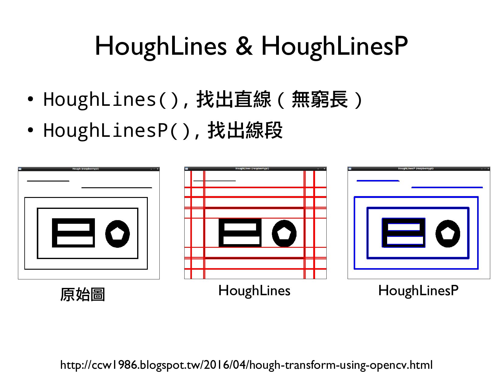
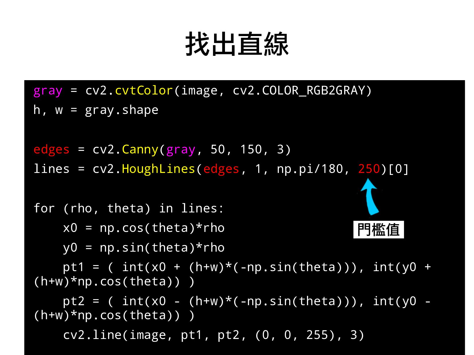
![• 原型 :cv2.HoughLines(image, rho, theta, threshold[, lines[, srn[, stn]]]) •](https://files.speakerdeck.com/presentations/79bbc2dc35484f3c9702a196c6f6cd5a/slide_93.jpg)
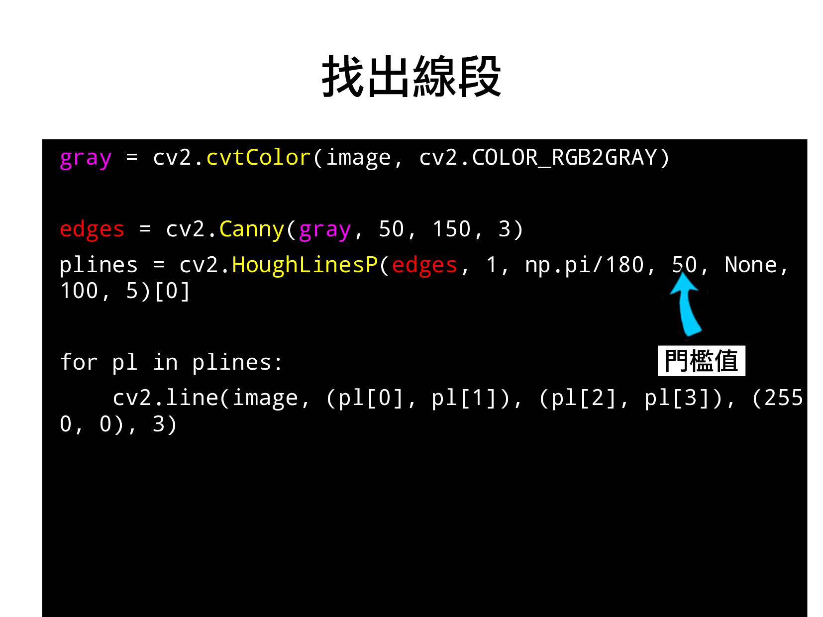
![• 原型 :cv2.HoughLinesP(image, rho, theta, threshold[, lines[, minLineLength[, maxLineGap]]]) •](https://files.speakerdeck.com/presentations/79bbc2dc35484f3c9702a196c6f6cd5a/slide_96.jpg)
![每組輪廓都可以找到找中心點 第一組輪廓點 cnt = contours[0] 第二組輪廓點 cnt = contours[1]](https://files.speakerdeck.com/presentations/79bbc2dc35484f3c9702a196c6f6cd5a/slide_109.jpg)
![faceCascade = cv2.CascadeClassifier(sys.argv[2]) image = cv2.imread(sys.argv[1]) gray = cv2.cvtColor(image, cv2.COLOR_BGR2GRAY)](https://files.speakerdeck.com/presentations/79bbc2dc35484f3c9702a196c6f6cd5a/slide_122.jpg)
![• 新進資料 [5, 8] 被分類到標籤 0( 紅色三角形 ) knn_static.py](https://files.speakerdeck.com/presentations/79bbc2dc35484f3c9702a196c6f6cd5a/slide_152.jpg)
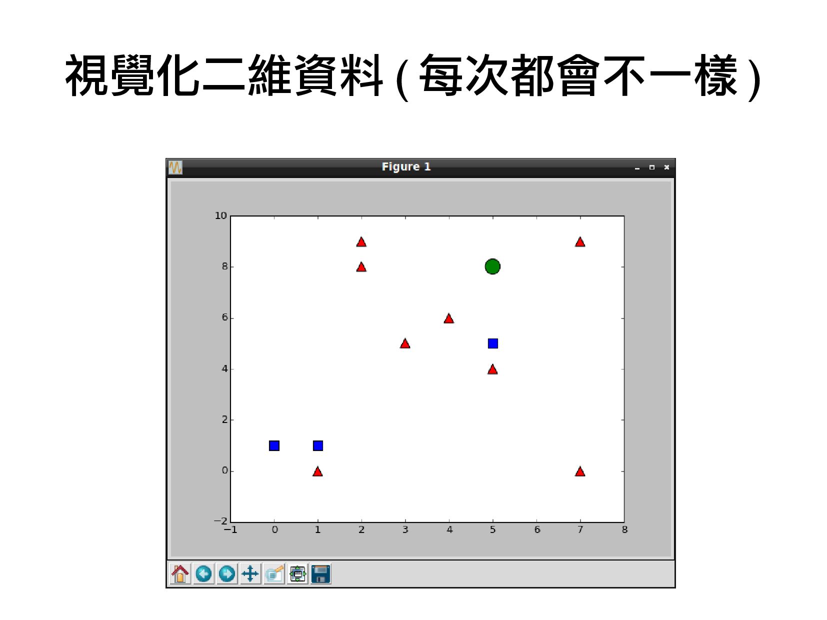
![• 新進資料 [5, 8] 被分類到標籤 0( 紅色三角形 ) knn_random.py (](https://files.speakerdeck.com/presentations/79bbc2dc35484f3c9702a196c6f6cd5a/slide_159.jpg)
![with np.load('knn_data.npz') as data: train = data['train'] train_labels = data['train_labels']](https://files.speakerdeck.com/presentations/79bbc2dc35484f3c9702a196c6f6cd5a/slide_173.jpg)
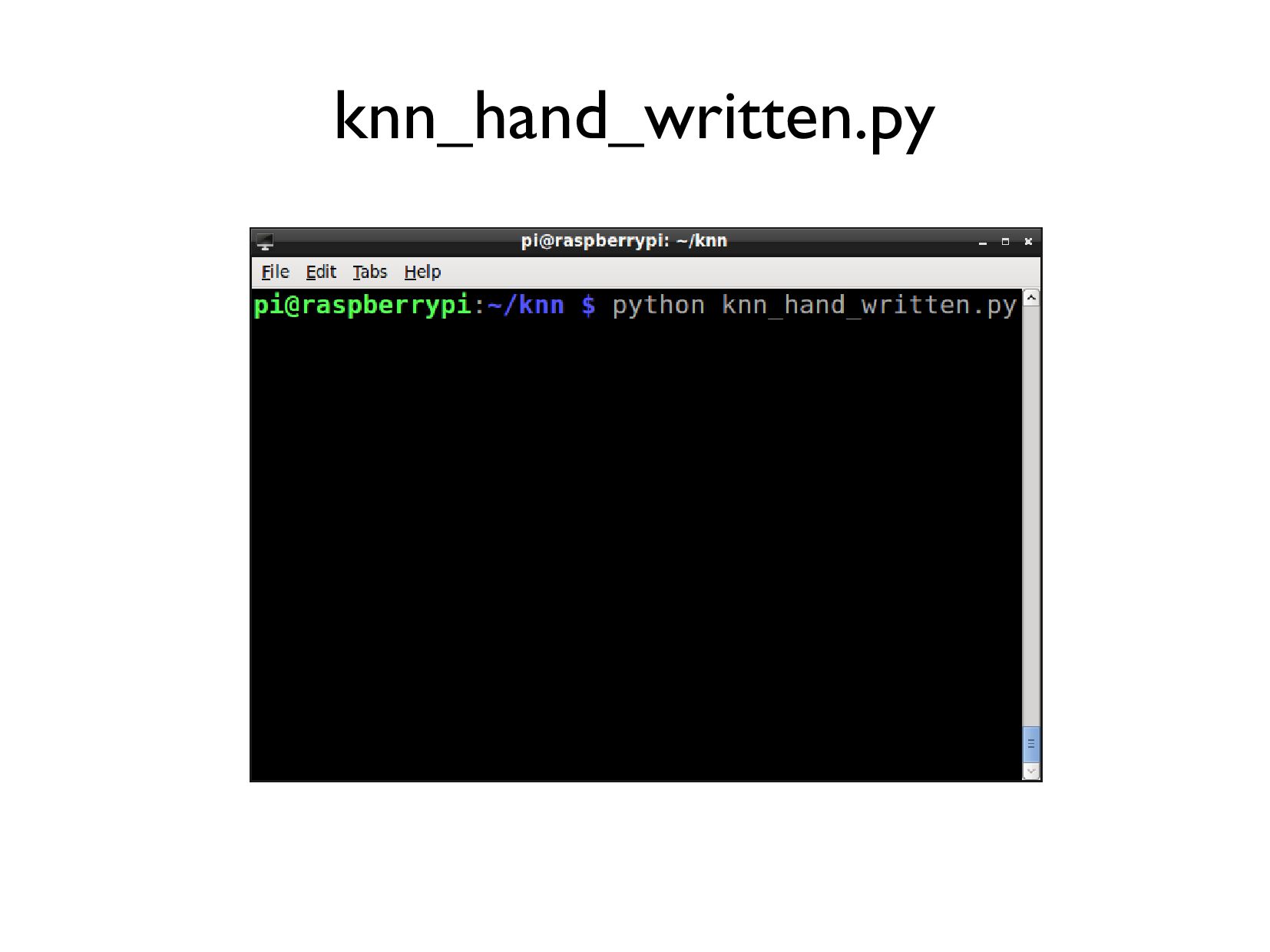