Christopher Fonnesbeck - Probabilistic Programming with PyMC3

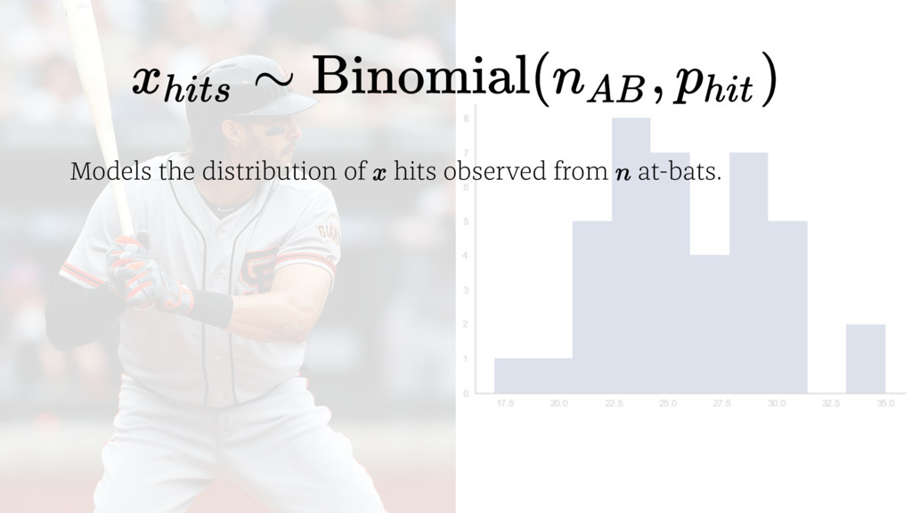
Bayesian statistics offers robust and flexible methods for data analysis that, because they are based on probability models, have the added benefit of being readily interpretable by non-statisticians. Until recently, however, the implementation of Bayesian models has been prohibitively complex for use by most analysts. But, the advent of probabilistic programming has served to abstract the complexity of Bayesian statistics, making such methods more broadly available. PyMC3 is a open-source Python module for probabilistic programming that implements several modern, computationally-intensive statistical algorithms for fitting Bayesian models, including Hamiltonian Monte Carlo (HMC) and variational inference. PyMC3’s intuitive syntax is helpful for new users, and the reliance on Theano for much of the computational work has allowed developers to keep the code base simple, making it easy to extend the software to meet analytic needs. PyMC3 itself extends Python's powerful "scientific stack" of development tools, which provide fast and efficient data structures, parallel processing, and interfaces for describing statistical models.

https://us.pycon.org/2017/schedule/presentation/473/

Transcript

1. Probabilistic Programming with Christopher Fonnesbeck Department of Biostatistics Vanderbilt University Medical Center
2. Probabilistic Programming
3. Stochastic language "primitives" Distribution over values: X ~ Normal(μ, σ) x = X.random(n=100) Distribution over functions: Y ~ GaussianProcess(mean_func(x), cov_func(x)) y = Y.predict(x2) Conditioning: p ~ Beta(1, 1) z ~ Bernoulli(p) # z|p
4. Bayesian Inference
5. Inverse Probability
6. Why Bayes? ❝The Bayesian approach is attractive because it is useful. Its usefulness derives in large measure from its simplicity. Its simplicity allows the investigation of far more complex models than can be handled by the tools in the classical toolbox.❞ —Link and Barker 2010
9. Probabilistic Programming in three easy steps
10. Encode a Probability Model⚐ 1 ⚐ in Python
11. Prior distribution Quantifies the uncertainty in latent variables
12. Prior distribution Quantifies the uncertainty in latent variables
13. Prior distribution Quantifies the uncertainty in latent variables
16. Likelihood function Conditions our model on the observed data
17. Likelihood function Conditions our model on the observed data
18. Models the distribution of hits observed from at-bats.
19. Counts per unit time
20. Infer Values for latent variables 2
21. Posterior distribution
22. Posterior distribution
23. Posterior distribution
24. Probabilistic programming abstracts the inference procedure
25. Check your Model 3
26. Model checking
27. WinBUGS
29. model { for (j in 1:J){ y[j] ~ dnorm (theta[j], tau.y[j]) theta[j] ~ dnorm (mu.theta, tau.theta) tau.y[j] <- pow(sigma.y[j], -2) } mu.theta ~ dnorm (0.0, 1.0E-6) tau.theta <- pow(sigma.theta, -2) sigma.theta ~ dunif (0, 1000) }
30. PyMC3 ☞ started in 2003 ☞ PP framework for fitting arbitrary probability models ☞ based on Theano ☞ implements "next generation" Bayesian inference methods ☞ NumFOCUS sponsored project !" github.com/pymc-devs/pymc3
31. Calculating Gradients in Theano >>> from theano import function, tensor as tt >>> x = tt.dmatrix('x') >>> s = tt.sum(1 / (1 + tt.exp(-x))) >>> gs = tt.grad(s, x) >>> dlogistic = function([x], gs) >>> dlogistic([[3, -1],[0, 2]]) array([[ 0.04517666, 0.19661193], [ 0.25 , 0.10499359]])
32. Calculating Gradients in Theano >>> from theano import function, tensor as tt >>> x = tt.dmatrix('x') >>> s = tt.sum(1 / (1 + tt.exp(-x))) >>> gs = tt.grad(s, x) >>> dlogistic = function([x], gs) >>> dlogistic([[3, -1],[0, 2]]) array([[ 0.04517666, 0.19661193], [ 0.25 , 0.10499359]])
33. Example: Radon exposure✴ ✴ Gelman et al. (2013) Bayesian Data Analysis
35. Unpooled model Model radon in each county independently. where (counties)
36. Priors with Model() as unpooled_model: α = Normal('α', 0, sd=1e5, shape=counties) β = Normal('β', 0, sd=1e5) σ = HalfCauchy('σ', 5)
37. >>> type(β) pymc3.model.FreeRV
38. >>> type(β) pymc3.model.FreeRV >>> β.distribution.logp(-2.1).eval() array(-12.4318639983954)
39. >>> type(β) pymc3.model.FreeRV >>> β.distribution.logp(-2.1).eval() array(-12.4318639983954) >>> β.random(size=4) array([ -10292.91760326, 22368.53416626, 124851.2516102, 44143.62513182]])
40. Transformed variables with unpooled_model: θ = α[county] + β*floor
41. Likelihood with unpooled_model: y = Normal('y', θ, sd=σ, observed=log_radon)
42. Model graph
43. Calculating Posteriors
46. Bayesian approximation ☞ Maximum a posteriori (MAP) estimate ☞ Laplace (normal) approximation ☞ Rejection sampling ☞ Importance sampling ☞ Sampling importance resampling (SIR) ☞ Approximate Bayesian Computing (ABC)
47. MCMC Markov chain Monte Carlo simulates a Markov chain for which some function of interest is the unique, invariant, limiting distribution.
48. MCMC Markov chain Monte Carlo simulates a Markov chain for which some function of interest is the unique, invariant, limiting distribution. This is guaranteed when the Markov chain is constructed that satisfies the detailed balance equation:
49. Metropolis sampling
50. Metropolis sampling** ** 2000 iterations, 1000 tuning
51. Hamiltonian Monte Carlo Uses a physical analogy of a frictionless particle moving on a hyper-surface Requires an auxiliary variable to be specified ☞ position (unknown variable value) ☞ momentum (auxiliary)
52. Hamiltonian MC ➀ Sample a new velocity from univariate Gaussian ➁ Perform n leapfrog steps to obtain new state ➂ Perform accept/reject move of
53. Hamiltonian MC** ** 2000 iterations, 1000 tuning
54. No U-Turn Sampler (NUTS) Hoffmann and Gelman (2014)
58. Variational Inference
59. Variational Inference Variational inference minimizes the Kullback-Leibler divergence from approximate distributions, but we can't calculate the true posterior distribution.
60. Evidence Lower Bound (ELBO)
61. ADVI* * Kucukelbir, A., Tran, D., Ranganath, R., Gelman, A., & Blei, D. M. (2016, March 2). Automatic Differentiation Variational Inference. arXiv.org.
62. Maximizing the ELBO
63. Estimating Beta(147, 255) posterior
64. with partial_pooling: approx = fit(n=100000) Average Loss = 1,115.5: 100%|██████████| 100000/100000 [00:13<00:00, 7690.51it/s] Finished [100%]: Average Loss = 1,115.5
65. with partial_pooling: approx = fit(n=100000) Average Loss = 1,115.5: 100%|██████████| 100000/100000 [00:13<00:00, 7690.51it/s] Finished [100%]: Average Loss = 1,115.5 >>> approx <pymc3.variational.approximations.MeanField at 0x119aa7c18>
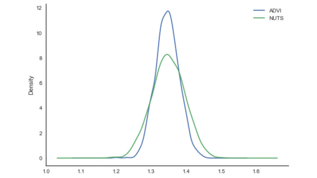
66. with partial_pooling: approx_sample = approx.sample(1000) traceplot(approx_sample, varnames=['mu_a', 'σ_a'])
68. New PyMC3 Features ☞ Gaussian processes ☞ Elliptical slice sampling ☞ Sequential Monte Carlo methods ☞ Time series models
69. Convolutional variational autoencoder♌ import keras class Decoder: ... def decode(self, zs): keras.backend.theano_backend._LEARNING_PHASE.set_value(np.uint8(0)) return self._get_dec_func()(zs) ♌ Taku Yoshioka (c) 2016
70. with pm.Model() as model: # Hidden variables zs = pm.Normal('zs', mu=0, sd=1, shape=(minibatch_size, dim_hidden), dtype='float32') # Decoder and its parameters dec = Decoder(zs, net=cnn_dec) # Observation model xs_ = pm.Normal('xs_', mu=dec.out.ravel(), sd=0.1, observed=xs_t.ravel(), dtype='float32')
71. Bayesian Deep Learning in PyMC3✧ ✧ Thomas Wiecki 2016
72. The Future ☞ Operator Variational Inference ☞ Normalizing Flows ☞ Riemannian Manifold HMC ☞ Stein variational gradient descent ☞ ODE solvers
73. Jupyter Notebook Gallery
75. The PyMC3 Team ☞ Colin Carroll ☞ Peadar Coyle ☞ Bill Engels ☞ Maxim Kochurov ☞ Junpeng Lao ☞ Osvaldo Martin ☞ Kyle Meyer ☞ Austin Rochford ☞ John Salvatier ☞ Adrian Seyboldt ☞ Thomas Wiecki ☞ Taku Yoshioka