Diving into Open Data with IPython Notebook & Pandas (Julia Evans)

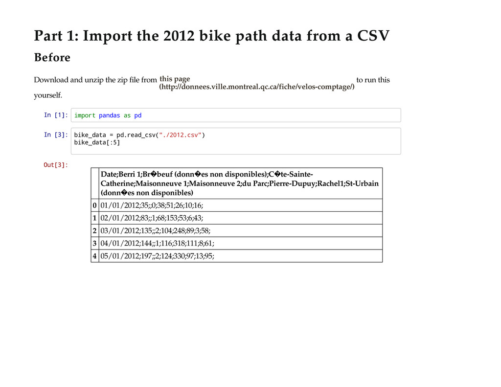
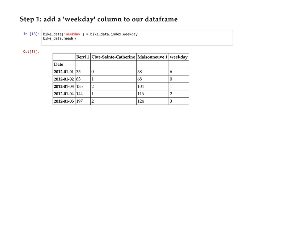
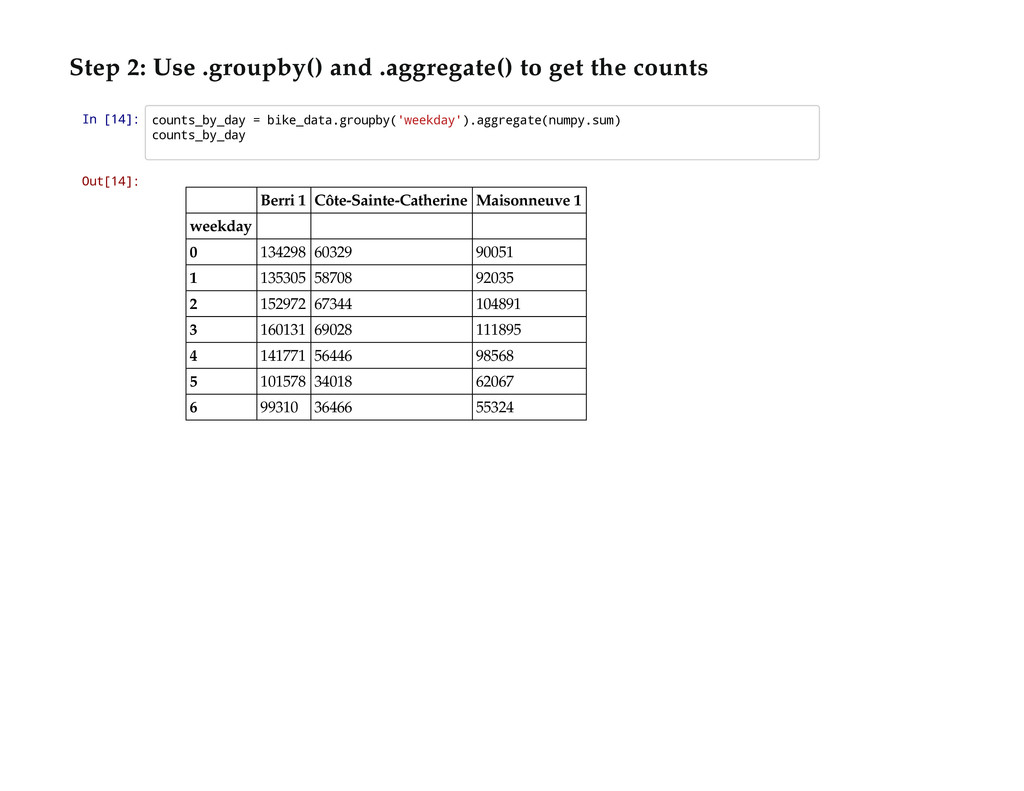
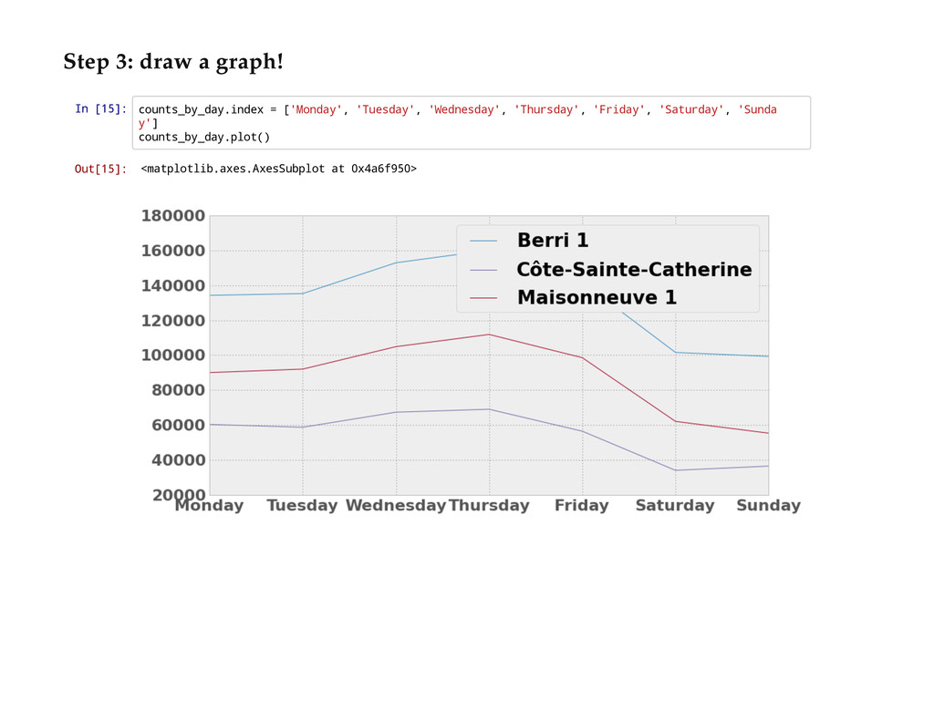
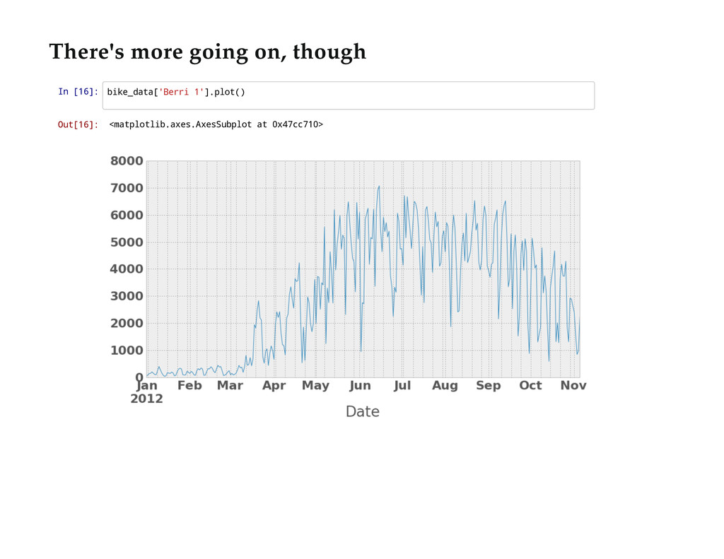
I'll walk you through Python's best tools for getting a grip on some new open data: IPython Notebook and pandas. I'll show you how to read in data, clean it up, graph it, and draw some conclusions, using some open data about the number of cyclists on Montréal's bike paths as an example.

Transcript

1. Diving into Open Data with IPython Notebook & Diving into Open Data with IPython Notebook & Pandas Pandas I'm Julia Evans I'm Julia Evans Data scientist, programmer, co-organize , You can follow along with this talk at: (http://twitter.com/b0rk) (http://jvns.ca) (http://github.com/jvns) (http://mtlallgirlhacknight.ca) (http://meetup.com/pyladiesmtl) (http://bit.ly/pyconca-pandas) http://bit.ly/pyconca-pandas PyLadies MTL Montréal All-Girl Hack Night http://github.com/jvns http://jvns.ca http://twitter.com/b0rk
2. IPython Notebook IPython Notebook web-based user interface to IPython pretty graphs literate programming Can make slideshows :) (this presentation) version controlled science! Pandas Pandas "R for Python" Provides easy to use data structures & a ton of useful helper functions for data cleanup and transformations Fast! (backed by numpy arrays) integrates well with scikit-learn
3. An installation warning An installation warning Don't: Use the Ubuntu packages Don't: Use the Ubuntu packages sudo apt-get install ipython-notebook sudo apt-get install python-pandas Do: Use pip or Do: Use pip or pip install ipython tornado pyzmq pip install pandas Anaconda is amazing. Anaconda is amazing. (https://store.continuum.io/) Anaconda
4. How to run IPython Notebook How to run IPython Notebook $ ipython notebook --pylab inline
5. The open data The open data Taken from (click "Vélos - comptage") Number of people per day on 7 bike paths (collected using sensors) (http://donnees.ville.montreal.qc.ca/) http://donnees.ville.montreal.qc.ca/fiche/velos-comptage/
6. Part 1: Import the 2012 bike path data from a CSV Part 1: Import the 2012 bike path data from a CSV Before Before Download and unzip the zip file from to run this yourself. In [1]: In [3]: (http://donnees.ville.montreal.qc.ca/fiche/velos-comptage/) import pandas as pd bike_data = pd.read_csv("./2012.csv") bike_data[:5] Out[3]: Date;Berri 1;Br�beuf (donn�es non disponibles);C�te-Sainte- Catherine;Maisonneuve 1;Maisonneuve 2;du Parc;Pierre-Dupuy;Rachel1;St-Urbain (donn�es non disponibles) 0 01/01/2012;35;;0;38;51;26;10;16; 1 02/01/2012;83;;1;68;153;53;6;43; 2 03/01/2012;135;;2;104;248;89;3;58; 3 04/01/2012;144;;1;116;318;111;8;61; 4 05/01/2012;197;;2;124;330;97;13;95; this page
7. After After In [4]: In [6]: Exercise: Parse the CSVs from 2011 and earlier (warning: it's annoying) bike_data = pd.read_csv("./2012.csv", encoding='latin1', sep=';', index_col='Date', pars e_dates=True, dayfirst=True) bike_data = bike_data[['Berri 1', u'Côte-Sainte-Catherine', 'Maisonneuve 1']] bike_data[:5] Out[6]: Berri 1 Côte-Sainte-Catherine Maisonneuve 1 Date 2012-01-01 35 0 38 2012-01-02 83 1 68 2012-01-03 135 2 104 2012-01-04 144 1 116 2012-01-05 197 2 124
8. Part 2: take a look at the data Part 2: take a look at the data We have a dataframe: In [7]: bike_data[:3] Out[7]: Berri 1 Côte-Sainte-Catherine Maisonneuve 1 Date 2012-01-01 35 0 38 2012-01-02 83 1 68 2012-01-03 135 2 104
9. In [8]: bike_data.plot() Out[8]: <matplotlib.axes.AxesSubplot at 0x3e59a90> /opt/anaconda/envs/ipython-1.0.0a1/lib/python2.7/site-packages/matplotlib/font_manager.py: 1224: UserWarning: findfont: Font family ['normal'] not found. Falling back to Bitstream V era Sans (prop.get_family(), self.defaultFamily[fontext]))
10. In [9]: bike_data.median() Out[9]: Berri 1 3128.0 Côte-Sainte-Catherine 1269.0 Maisonneuve 1 2019.5 dtype: float64
11. In [10]: bike_data.median().plot(kind='bar') Out[10]: <matplotlib.axes.AxesSubplot at 0x3fd98d0>
13. Slicing dataframes Slicing dataframes In [11]: # column slice column_slice = bike_data[['Berri 1', 'Maisonneuve 1']] # row slice column_slice[:3] Out[11]: Berri 1 Maisonneuve 1 Date 2012-01-01 35 38 2012-01-02 83 68 2012-01-03 135 104
14. In [12]: column_slice.plot() Out[12]: <matplotlib.axes.AxesSubplot at 0x43bcbd0>
15. Part 2: Do more people bike on weekdays or Part 2: Do more people bike on weekdays or weekends? weekends?
16. Step 1: add a 'weekday' column to our dataframe Step 1: add a 'weekday' column to our dataframe In [13]: bike_data['weekday'] = bike_data.index.weekday bike_data.head() Out[13]: Berri 1 Côte-Sainte-Catherine Maisonneuve 1 weekday Date 2012-01-01 35 0 38 6 2012-01-02 83 1 68 0 2012-01-03 135 2 104 1 2012-01-04 144 1 116 2 2012-01-05 197 2 124 3
17. Step 2: Use .groupby() and .aggregate() to get the counts Step 2: Use .groupby() and .aggregate() to get the counts In [14]: counts_by_day = bike_data.groupby('weekday').aggregate(numpy.sum) counts_by_day Out[14]: Berri 1 Côte-Sainte-Catherine Maisonneuve 1 weekday 0 134298 60329 90051 1 135305 58708 92035 2 152972 67344 104891 3 160131 69028 111895 4 141771 56446 98568 5 101578 34018 62067 6 99310 36466 55324
18. Step 3: draw a graph! Step 3: draw a graph! In [15]: counts_by_day.index = ['Monday', 'Tuesday', 'Wednesday', 'Thursday', 'Friday', 'Saturday', 'Sunda y'] counts_by_day.plot() Out[15]: <matplotlib.axes.AxesSubplot at 0x4a6f950>
19. There's more going on, though There's more going on, though In [16]: bike_data['Berri 1'].plot() Out[16]: <matplotlib.axes.AxesSubplot at 0x47cc710>
20. Part 3: Grab some weather data and look at the Part 3: Grab some weather data and look at the temperatures temperatures In [17]: In [18]: def get_weather_data(year): url_template = "http://climate.weather.gc.ca/climateData/bulkdata_e.html?format=csv& stationID=5415&Year={year}&Month={month}&timeframe=1&submit=Download+Data" # mctavish station: 10761, airport station: 5415 data_by_month = [] for month in range(1, 13): url = url_template.format(year=year, month=month) weather_data = pd.read_csv(url, skiprows=16, index_col='Date/Time', parse_dates= True).dropna(axis=1) weather_data.columns = map(lambda x: x.replace('\xb0', ''), weather_data.columns ) weather_data = weather_data.drop(['Year', 'Day', 'Month', 'Time', 'Data Quality' ], axis=1) data_by_month.append(weather_data.dropna()) # Concatenate and drop any empty columns return pd.concat(data_by_month).dropna(axis=1, how='all').dropna() weather_data = get_weather_data(2012)
21. In [19]: weather_data[:5] Out[19]: Dew Point Temp (C) Rel Hum (%) Stn Press (kPa) Temp (C) Visibility (km) Weather Wind Spd (km/h) Date/Time 2012-01-01 00:00:00 -3.9 86 101.24 -1.8 8.0 Fog 4 2012-01-01 01:00:00 -3.7 87 101.24 -1.8 8.0 Fog 4 2012-01-01 02:00:00 -3.4 89 101.26 -1.8 4.0 Freezing Drizzle,Fog 7 2012-01-01 03:00:00 -3.2 88 101.27 -1.5 4.0 Freezing Drizzle,Fog 6 2012-01-01 04:00:00 -3.3 88 101.23 -1.5 4.8 Fog 7
22. We need the temperatures every day, not every hour... We need the temperatures every day, not every hour... In [20]: In [21]: bike_data['mean temp'] = weather_data['Temp (C)'].resample('D', how='mean') bike_data.head() Out[21]: Berri 1 Côte-Sainte-Catherine Maisonneuve 1 weekday mean temp Date 2012-01-01 35 0 38 6 0.629167 2012-01-02 83 1 68 0 0.041667 2012-01-03 135 2 104 1 -14.416667 2012-01-04 144 1 116 2 -13.645833 2012-01-05 197 2 124 3 -6.750000
23. Bikers per day and temperature Bikers per day and temperature In [22]: bike_data[['Berri 1', 'mean temp']].plot(subplots=True) Out[22]: array([<matplotlib.axes.AxesSubplot object at 0x52efed0>, <matplotlib.axes.AxesSubplot object at 0x5525a90>], dtype=object)
24. Do people bike when it's raining? Do people bike when it's raining? In [23]: bike_data['Rain'] = weather_data['Weather'].str.contains('Rain').map(lambda x: int(x)).r esample('D', how='mean')
25. In [24]: bike_data[['Berri 1', 'Rain']].plot(subplots=True) Out[24]: array([<matplotlib.axes.AxesSubplot object at 0x5900b10>, <matplotlib.axes.AxesSubplot object at 0x6289ed0>], dtype=object)
26. Let's look at unpopular days in the summer Let's look at unpopular days in the summer In [25]: In [26]: # Look at everything between May and September summertime_data = bike_data['2012-05-01':'2012-09-01'] summertime_data['Berri 1'][:5] < 2500 Out[26]: Date 2012-05-01 True 2012-05-02 False 2012-05-03 False 2012-05-04 False 2012-05-05 False Name: Berri 1, dtype: bool
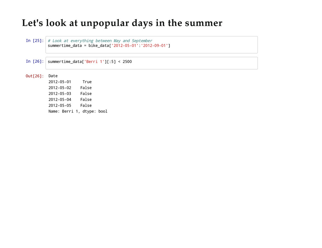
27. In [27]: summertime_data = bike_data['2012-05-01':'2012-09-01'] bad_days = summertime_data[summertime_data['Berri 1'] < 2500] bad_days[['Berri 1', 'Rain', 'mean temp', 'weekday']] Out[27]: Berri 1 Rain mean temp weekday Date 2012-05-01 1986 0.416667 9.437500 1 2012-05-08 1241 0.666667 12.645833 1 2012-05-22 2315 0.583333 18.279167 1 2012-06-02 943 0.583333 13.566667 5 2012-06-25 2245 0.208333 17.270833 0 2012-08-05 1864 0.166667 25.783333 6 2012-08-10 2414 0.458333 19.841667 4 2012-08-11 2453 0.125000 20.891667 5
28. Some advice Some advice Read (some of) the documentation has a 460-page PDF with lots of examples Python for Data Analysis by Wes McKinney is great Always use vectorized operations, try not to write your own loops (though: see Numba) (http://pandas.pydata.org/) http://pandas.pydata.org/
29. Thanks! Questions? Thanks! Questions? In [29]: print 'Email:', julia['email'] print 'Twitter:', julia['twitter'] print 'Slides: http://bit.ly/pyconca-pandas' Email: julia@jvns.ca Twitter: http://twitter.com/b0rk Slides: http://bit.ly/pyconca-pandas