Numerical Approaches to Holography

Transcript

1. NUMERICAL APPROACHES TO HOLOGRAPHY Talk online at - raghavgjha.net IISER Mohali Raghav Govind Jha 08.08.2019 (from 01.09.2019) !1
2. Overview !2 1. Holographic principle (AdS/CFT) and generalizations. 2. Lattice discretization of a ‘supersymmetric’ field theory (N=4 SYM) PART-II 3. Numerical Approach to holography using tensor networks. 4. Tensor network formulation of a 2d gauge-Higgs system. 5. Conclusions
3. Some remarks! !3 The numbers (format YYMM.XXXXX) quoted for reference are the arXiv numbers. You can search for those papers on www.arxiv.org SYM = Supersymmetric Yang-Mills. An example of field theory which is supersymmetric (i.e. the bosonic terms and fermionic terms are related by some symmetry). This is a very special property. No experimental evidence. Field theory — Combination of classical field theory, special relativity, and quantum mechanics. For ex. - QED (Quantum Electrodynamics) is a relativistic quantum field theory of electrodynamics and deals with interactions of photons with matter.
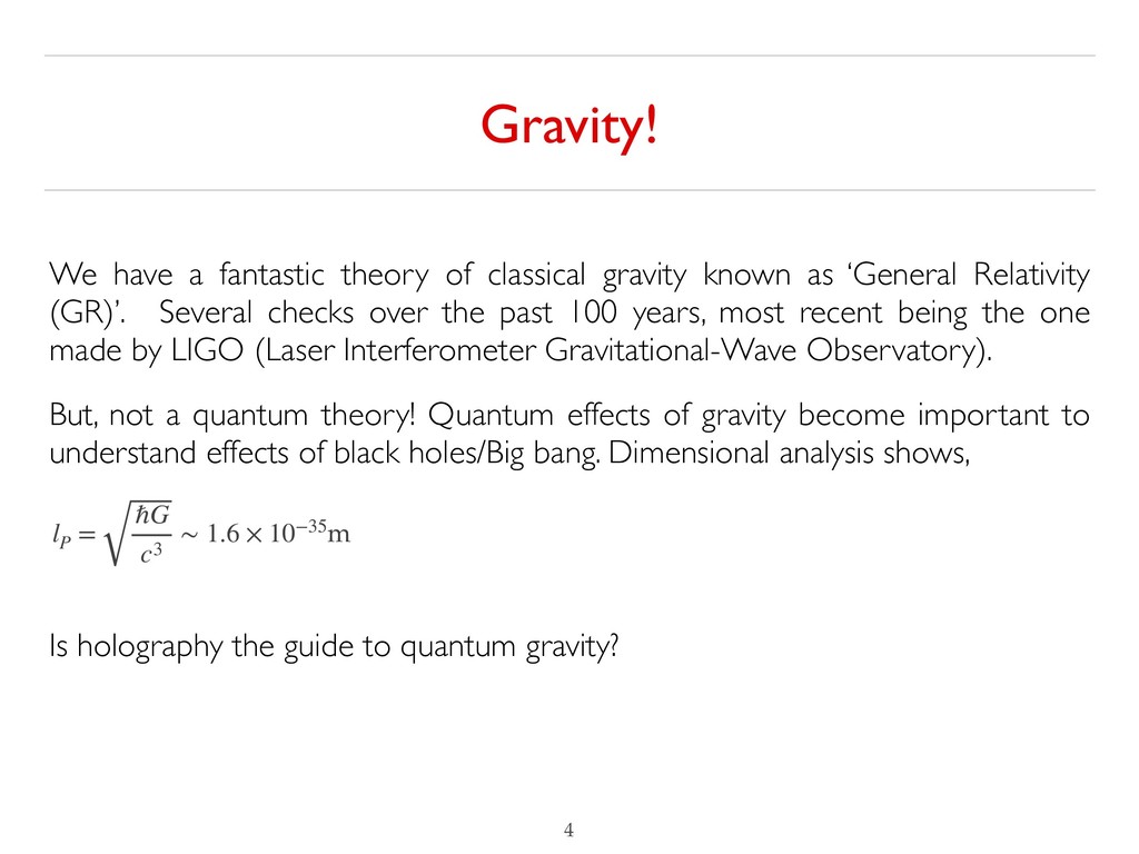
4. Gravity! !4 We have a fantastic theory of classical gravity known as ‘General Relativity (GR)’. Several checks over the past 100 years, most recent being the one made by LIGO (Laser Interferometer Gravitational-Wave Observatory). But, not a quantum theory! Quantum effects of gravity become important to understand effects of black holes/Big bang. Dimensional analysis shows, Is holography the guide to quantum gravity? lP = ℏG c3 ∼ 1.6 × 10−35m
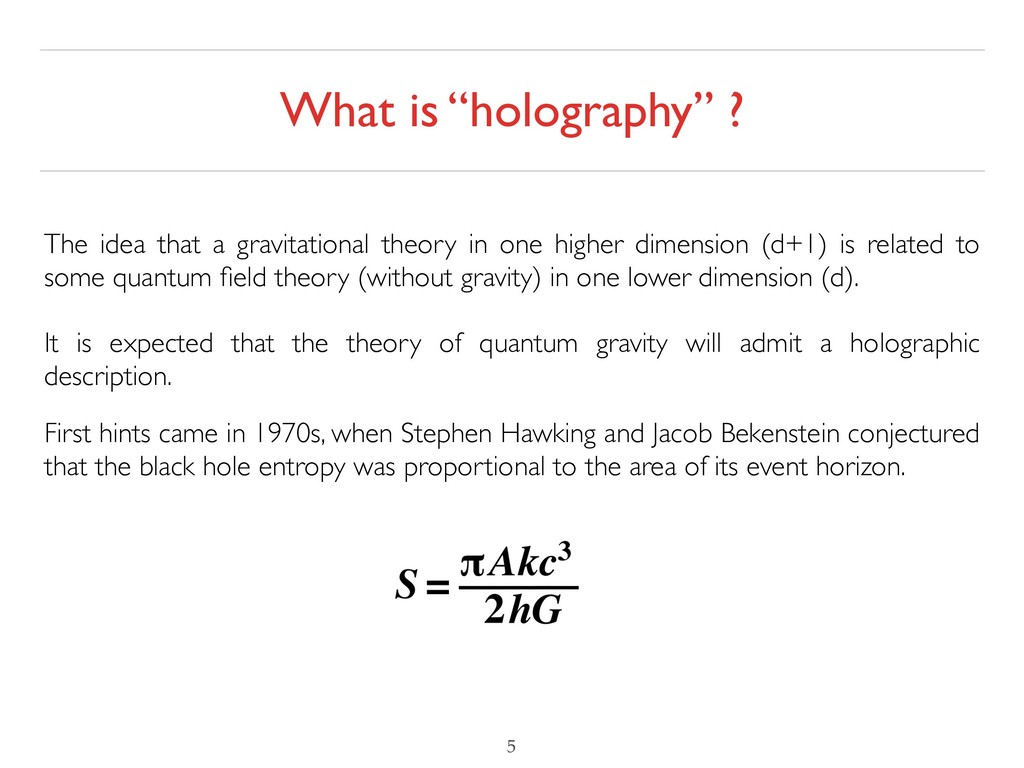
5. What is “holography” ? !5 The idea that a gravitational theory in one higher dimension (d+1) is related to some quantum field theory (without gravity) in one lower dimension (d). 
 
 It is expected that the theory of quantum gravity will admit a holographic description. First hints came in 1970s, when Stephen Hawking and Jacob Bekenstein conjectured that the black hole entropy was proportional to the area of its event horizon.
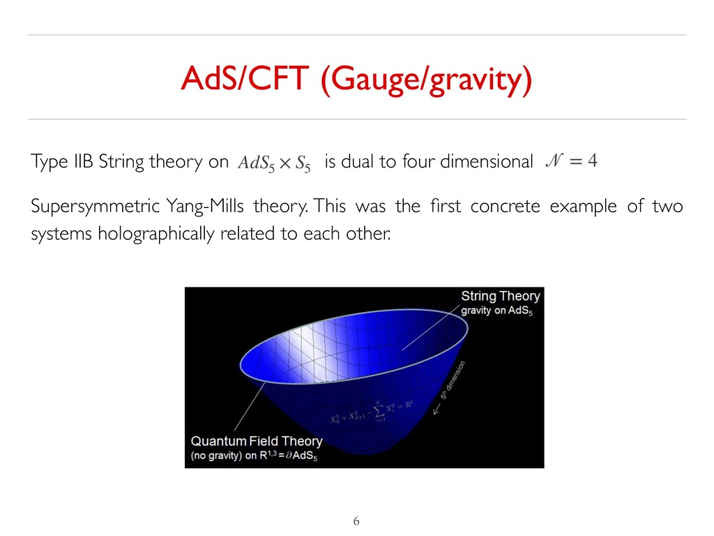
6. AdS/CFT (Gauge/gravity) !6 Type IIB String theory on is dual to four dimensional Supersymmetric Yang-Mills theory. This was the first concrete example of two systems holographically related to each other. AdS5 × S5 = 4
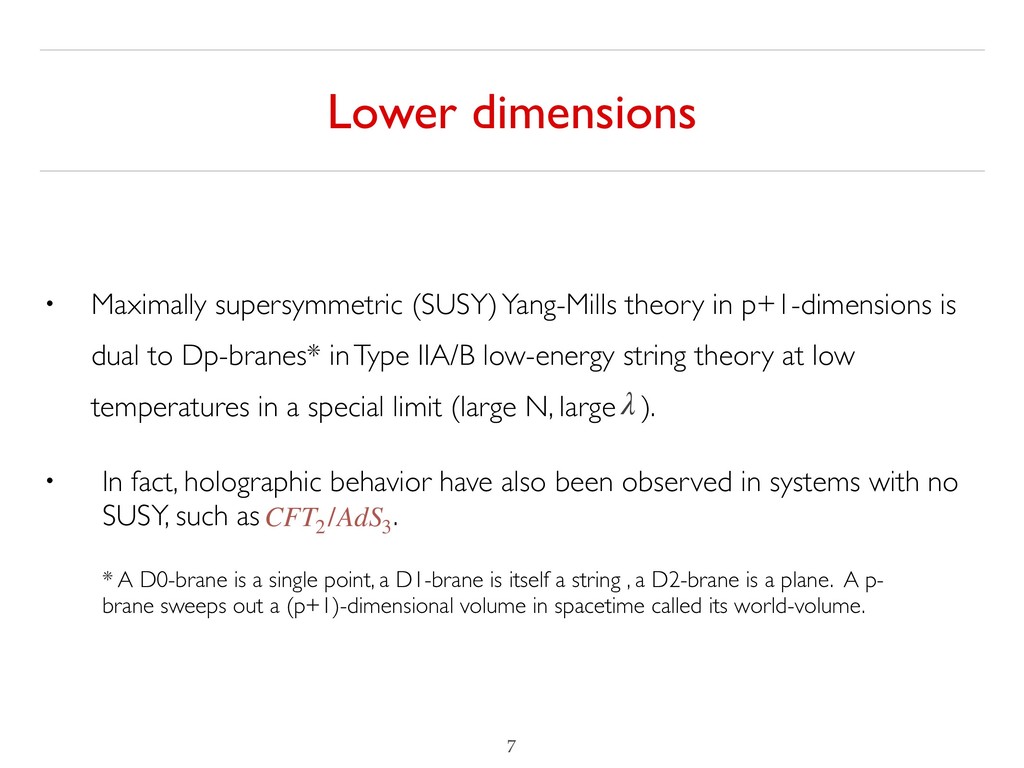
7. Lower dimensions !7 • Maximally supersymmetric (SUSY) Yang-Mills theory in p+1-dimensions is dual to Dp-branes* in Type IIA/B low-energy string theory at low temperatures in a special limit (large N, large ). • In fact, holographic behavior have also been observed in systems with no SUSY, such as . 
 
 * A D0-brane is a single point, a D1-brane is itself a string , a D2-brane is a plane. A p- brane sweeps out a (p+1)-dimensional volume in spacetime called its world-volume. λ CFT2 /AdS3
8. No proof … a weak/strong conjecture! !8 Even though AdS/CFT or more generally gauge/gravity is a wonderful idea connecting two different theories in different dimensions, it has no proof. Need to rigorously test this conjecture has led to lot of interesting work.
9. Beyond perturbation theory - Numerics !9 Any non-trivial proof of the conjecture has to systematically handle strong coupling limit. We know from our experience of theory of strong interactions (QCD) that lattice methods can be useful. Natural to apply this tool in this context. We also need large N limit, i.e. the gauge group is SU(N), where N is large.
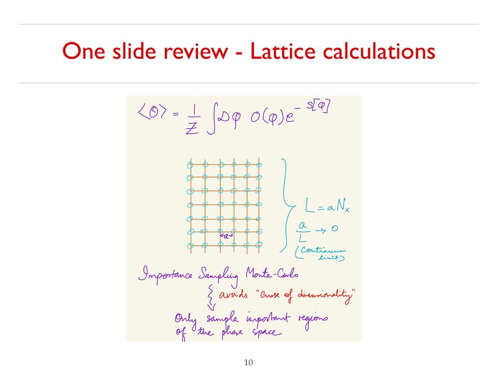
10. One slide review - Lattice calculations !10 ⑧ = ¥ fog o (g) e- she] 0*000 0000-00 000-000 :¥¥÷¥÷¥is÷ : " - continuing Importance Sampling Monte-Carlo { avoids " curse of dimensionality " Only sample important regions of the phase space
11. Phase space for SYM/QCD !11
12. =4 SYM theory !12 Most of the holographic predictions are related to this theory or its dimensional reductions. It is important to study this theory numerically in the strong coupling limit. This has led to the field of lattice SYM. For a review see, 0903.4881 = 4
13. =4 SYM theory !13 Obtained by dimensionally reducing the ten-dimensional SYM theory down to four dimensions. Conformal field theory, beta-function vanishes, consists of six scalars, sixteen real fermions, all massless and in the adjoint representation of the SU(N) gauge group. In the limit of large N, this has a well-defined holographic dual which gives rise to black holes in Type IIB supergravity (SUGRA).
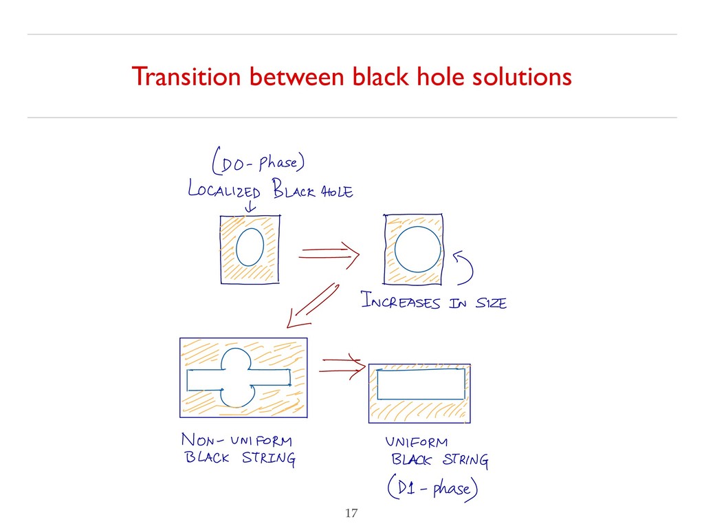
14. Dimensionally reduced SYMs !14 • Reduce the theory to (1+1)-dimensions to study SYM theory dual to Type IIB SUGRA having different black hole solutions (uniform black string and localised black hole) and transition between them. • Reduce the four dimensional theory down to one dimension (0+1, time, SQM) to get BFSS (Banks-Fischler-Shenker-Susskind) model. • Add mass deformation to this theory to study matrix model on pp-wave space-time, known as BMN (Berenstein-Maldacena-Nastase) model.
15. Regime of supergravity validity (p<3) !15 α′ λ gs ≪ 1 1 ≪ λp β3−p ≪ N 10 − 2p 7 − p To have a valid SUGRA limit, we need: • Radius of curvature large in units of , which means T << 1 or >> 1 • The string coupling, , which means that N should be large. These two combined gives the following : , note that for p=3, this reduces to the familiar limit.
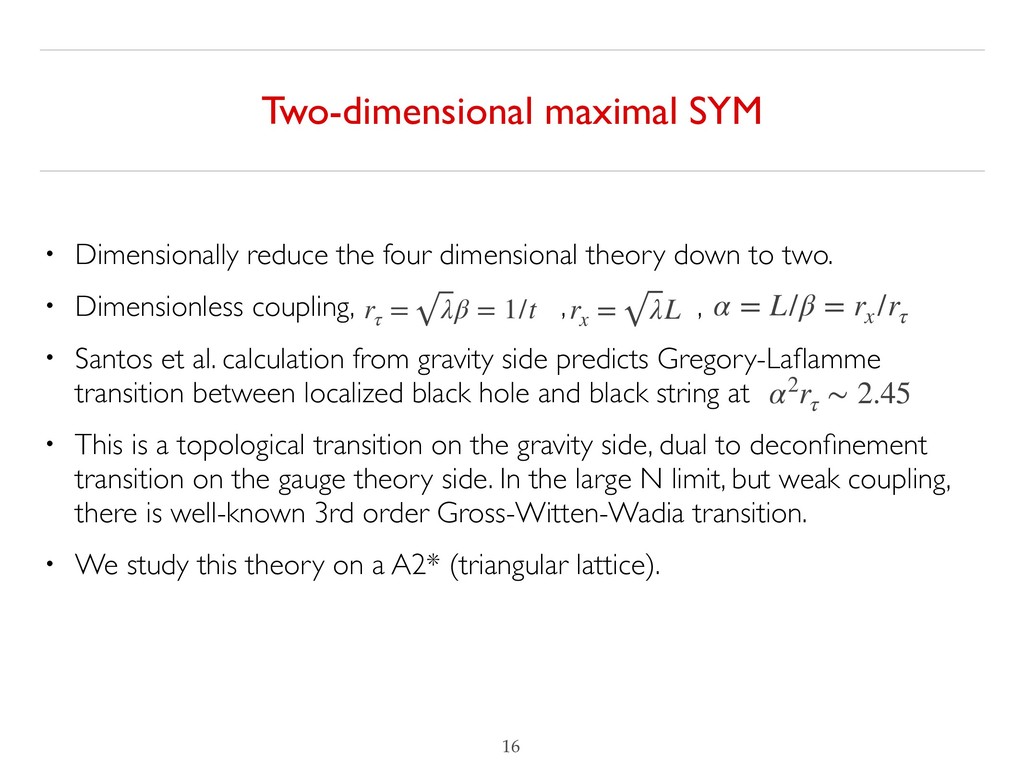
16. Two-dimensional maximal SYM !16 rτ = λβ = 1/t rx = λL α = L/β = rx /rτ α2rτ ∼ 2.45 • Dimensionally reduce the four dimensional theory down to two. • Dimensionless coupling, , , • Santos et al. calculation from gravity side predicts Gregory-Laflamme transition between localized black hole and black string at • This is a topological transition on the gravity side, dual to deconfinement transition on the gauge theory side. In the large N limit, but weak coupling, there is well-known 3rd order Gross-Witten-Wadia transition. • We study this theory on a A2* (triangular lattice).
17. Transition between black hole solutions !17 (DO - phase ) LOCALIZED BLACK HOLE EEEEIE : 㱺 # INCREASES IN SIZE No FIFE't , " III. " Tanna (D1 - phase)
18. Results - I 
 Phys. Rev. D 97, 086020 (2018), 1709.07025 !18 gravity D0-phase gravity D1-phase Deconfinement transition Deconfinement transition BQM limit gravity limit ? r3 L = cBQM r r2 L = cgravr PL = 0 PL 6= 0 rL r
19. Results - II 
 Phys. Rev. D 97, 086020 (2018), 1709.07025 !19
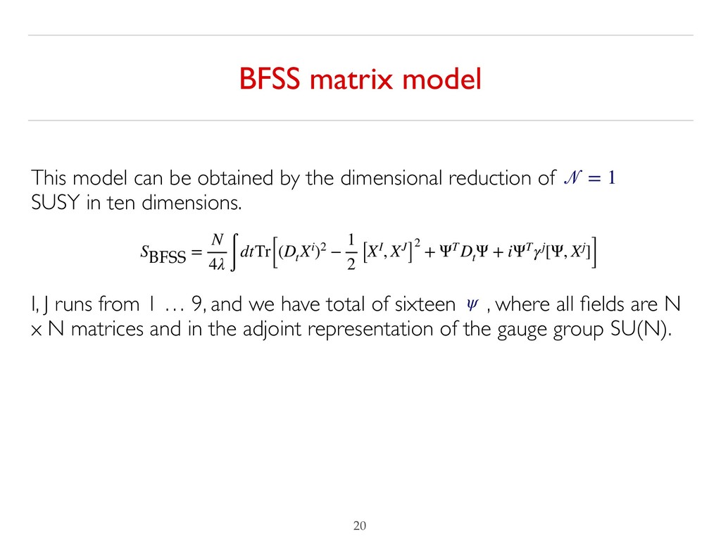
20. BFSS matrix model !20 This model can be obtained by the dimensional reduction of SUSY in ten dimensions. I, J runs from 1 … 9, and we have total of sixteen , where all fields are N x N matrices and in the adjoint representation of the gauge group SU(N). SBFSS = N 4λ ∫ dtTr[(Dt Xi)2 − 1 2 [XI, XJ] 2 + ΨTDt Ψ + iΨTγj[Ψ, Xj]] = 1 ψ
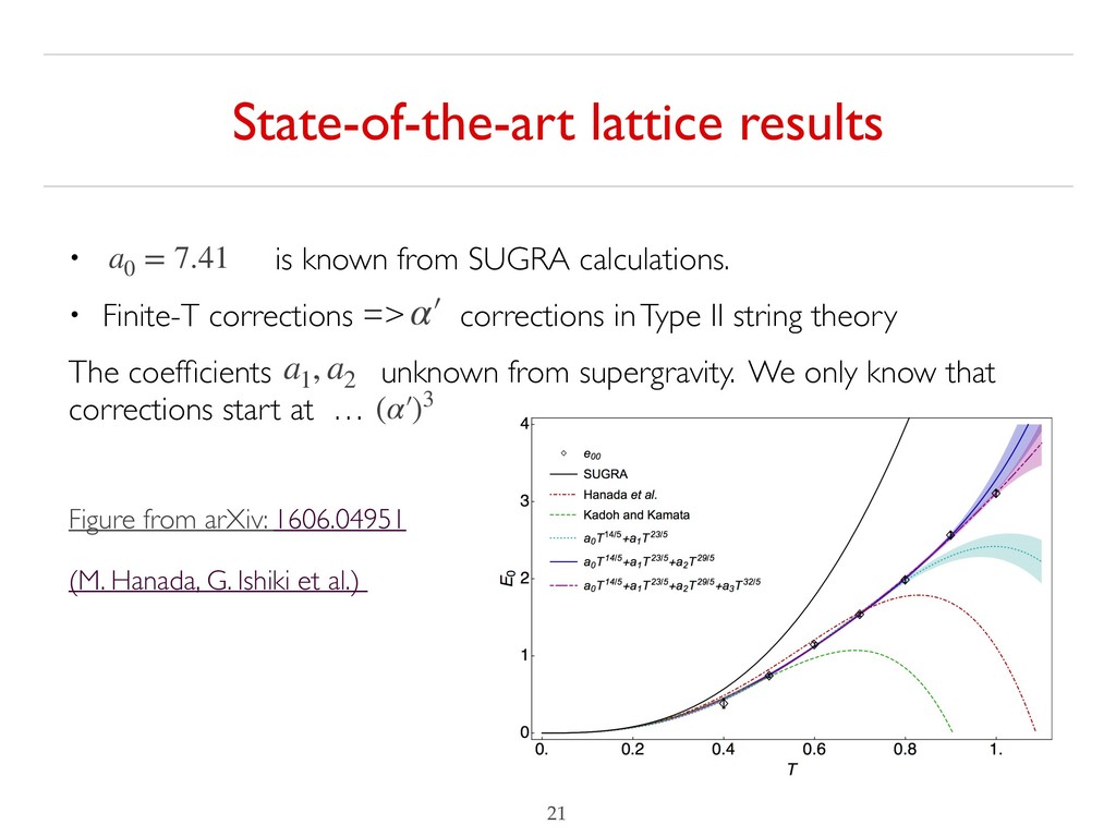
21. State-of-the-art lattice results !21 a0 = 7.41 α′ a1 , a2 (α′)3 • is known from SUGRA calculations. • Finite-T corrections => corrections in Type II string theory The coefficients unknown from supergravity. We only know that corrections start at … Figure from arXiv: 1606.04951 (M. Hanada, G. Ishiki et al.)
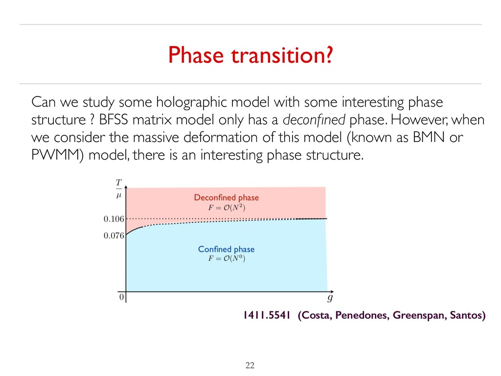
22. Phase transition? !22 Can we study some holographic model with some interesting phase structure ? BFSS matrix model only has a deconfined phase. However, when we consider the massive deformation of this model (known as BMN or PWMM) model, there is an interesting phase structure. 1411.5541 (Costa, Penedones, Greenspan, Santos)
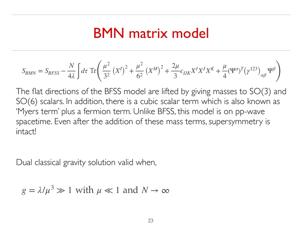
23. BMN matrix model !23 SBMN = SBFSS − N 4λ ∫ dτ Tr ( μ2 32 (XI) 2 + μ2 62 (XM) 2 + 2μ 3 ϵIJK XI XJXK + μ 4 (Ψα)T(γ123) αβ Ψβ ) g = λ/μ3 ≫ 1 with μ ≪ 1 and N → ∞ The flat directions of the BFSS model are lifted by giving masses to SO(3) and SO(6) scalars. In addition, there is a cubic scalar term which is also known as ‘Myers term’ plus a fermion term. Unlike BFSS, this model is on pp-wave spacetime. Even after the addition of these mass terms, supersymmetry is intact! Dual classical gravity solution valid when,
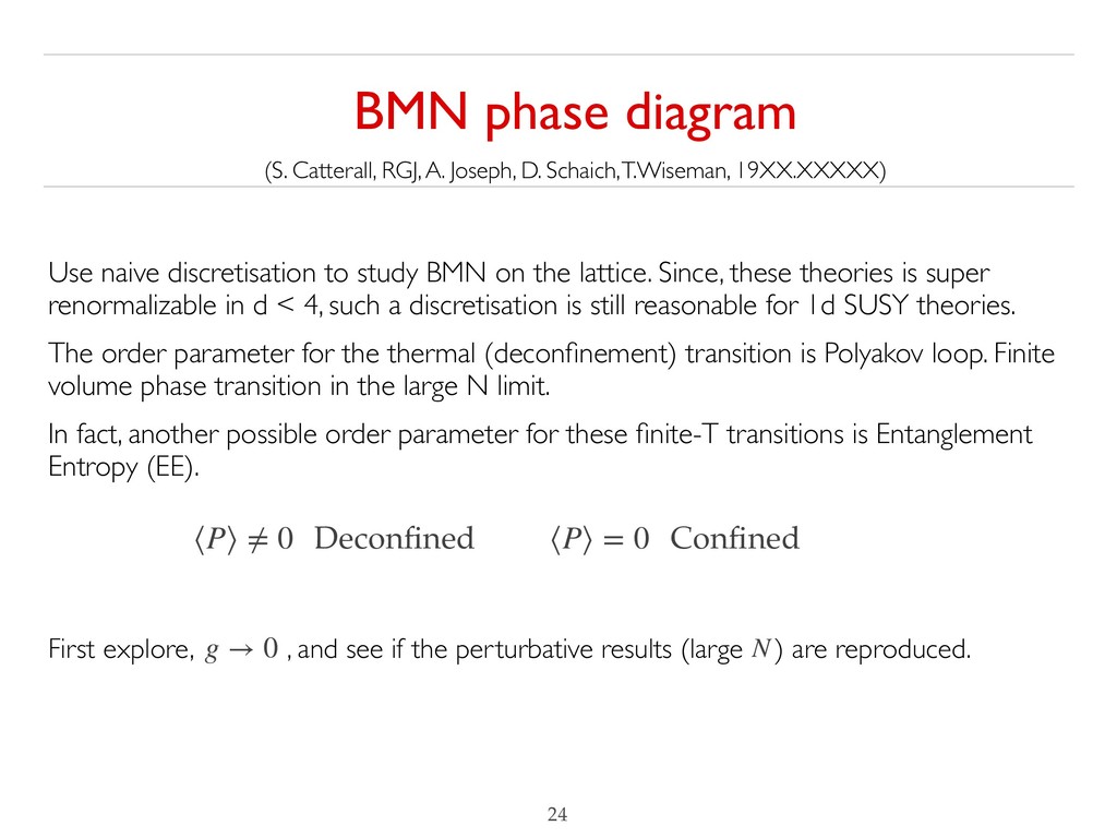
24. !24 g → 0 N ⟨P⟩ ≠ 0 Deconfined ⟨P⟩ = 0 Confined Use naive discretisation to study BMN on the lattice. Since, these theories is super renormalizable in d < 4, such a discretisation is still reasonable for 1d SUSY theories. The order parameter for the thermal (deconfinement) transition is Polyakov loop. Finite volume phase transition in the large N limit. In fact, another possible order parameter for these finite-T transitions is Entanglement Entropy (EE). First explore, , and see if the perturbative results (large ) are reproduced. BMN phase diagram (S. Catterall, RGJ, A. Joseph, D. Schaich, T.Wiseman, 19XX.XXXXX)
25. BMN phase diagram ... continued
 (S. Catterall, RGJ, A. Joseph, D. Schaich, T.Wiseman, 19XX.XXXXX) !25 such Polyakov loop as order parameter Finite coupling phase transition from lattice calculations.
26. Ongoing & future work in 3d SYM and N=4 SYM 
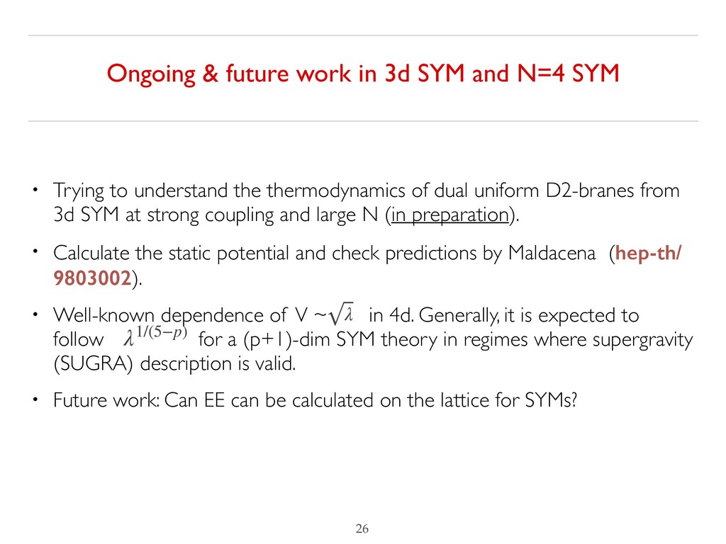
 !26 • Trying to understand the thermodynamics of dual uniform D2-branes from 3d SYM at strong coupling and large N (in preparation). • Calculate the static potential and check predictions by Maldacena (hep-th/ 9803002). • Well-known dependence of V ~ in 4d. Generally, it is expected to follow for a (p+1)-dim SYM theory in regimes where supergravity (SUGRA) description is valid. • Future work: Can EE can be calculated on the lattice for SYMs? λ λ1/(5−p)
27. *Tensor networks* !27 Several motivations to study tensor networks 1. Expected to play fundamental role in putting AdS/CFT on a firm footing via understanding the properties (geometry) of the bulk physics from entangled quantum state. *Brief mention 2. Provides an arena for studying lower-dimensional critical 
 systems (faster and more efficiently) than any other method 3. Possibility of formulating gauge theories in terms of
 tensors can enable us to study theories where usual Monte Carlo methods fail [sign problems!] *Some results
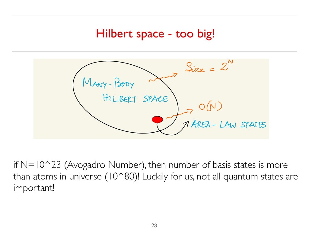
28. Hilbert space - too big! !28 if N=10^23 (Avogadro Number), then number of basis states is more than atoms in universe (10^80)! Luckily for us, not all quantum states are important! -7 Size = 2N ¥¥i⾨÷ .in?uws.i*es The region of ' H' that obeys the area - law scaling for the entanglement entropy corresponds to a tiny corner of the entire space . IMAGINE : N ~ 9023 ( order of Avogadro Number ) , the number of basis States is FL is more
29. Many-body ground state !29 Ground states are not “arbitrary” states in Hilbert space, it has very special features. Some of which have been captured by studying the entanglement entropy (EE). The region of Hilbert space that obeys area-law scaling for the EE corresponds to a tiny corner. Therefore, lot of progress have been made in many-body physics by finding EE and hence identifying important regions of Hilbert space.
30. Classes of local Hamiltonian !30 DMRG Gapped/ Non- Critical Gapless/ Critical ℋ C(x1 , x2 ) S(A)1+1d ∼ exp[(x1 − x2 )/ξ] ∼ |x1 − x2 |−q S is the entanglement entropy associated with some region A, ξ ≥ 0 is the correlation length, q ≥ 0 ∼ L0 ∼ constant ln(LA )
31. AdS/MERA !31 Based on these observations, several tensor networks have been proposed which tries to capture the ground state wave function of the system near critical point or away from it. One such tensor network which is used to describe critical systems (with ‘log’ scaling of EE) is called multi-scale entanglement ansatz (MERA) and it efficiently captures the ground state of the critical systems (which are CFTs in field theory language). (Figure courtesy: 1106.1082)
32. Different tensor networks !32 MPS (Matrix Product States) with open boundary condition (OBC) and periodic boundary conditions (PBC), Figure: 1306.2164 PEPS (Projected Entangled Pair States) Scale invariant MERA, Figure: 1106.1082
33. Basics of Tensor indices! !33 Figure: 1112.4101
34. 2d non-Abelian gauge+Higgs model 
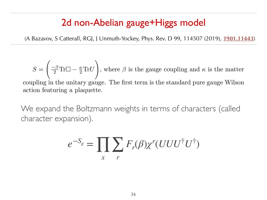
 (A Bazavov, S Catterall, RGJ, J Unmuth-Yockey, Phys. Rev. D 99, 114507 (2019), 1901.11443) !34 S = 2 Tr⇤  2 TrU ! , where is the gauge coupling and  is the matter coupling in the unitary gauge. The first term is the standard pure gauge Wilson action featuring a plaquette. We expand the Boltzmann weights in terms of characters (called character expansion). e−Sg = ∏ x ∑ r Fr (β)χr(UUU†U†)
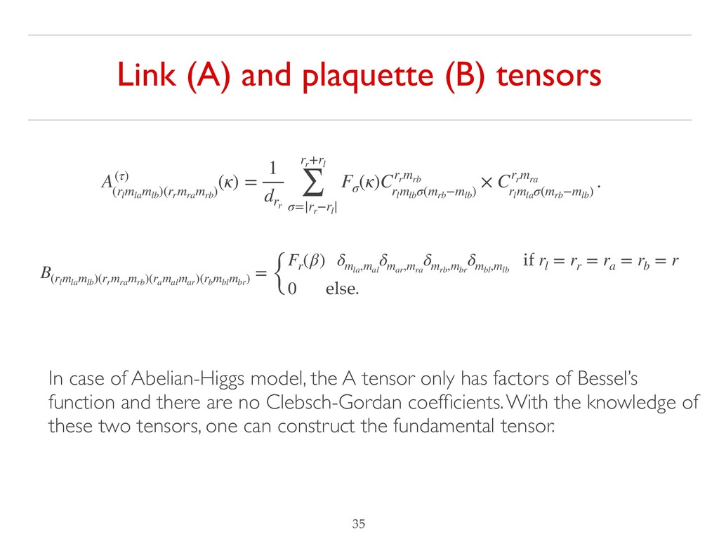
35. Link (A) and plaquette (B) tensors !35 A(τ) (rl mla mlb )(rr mra mrb ) (κ) = 1 drr rr +rl ∑ σ=|rr −rl | Fσ (κ)Crr mrb rl mlb σ(mrb −mlb ) × Crr mra rl mla σ(mrb −mlb ) . B(rl mla mlb )(rr mra mrb )(ra mal mar )(rb mbl mbr ) = { Fr (β) δmla ,mal δmar ,mra δmrb ,mbr δmbl ,mlb if rl = rr = ra = rb = r 0 else. In case of Abelian-Higgs model, the A tensor only has factors of Bessel’s function and there are no Clebsch-Gordan coefficients. With the knowledge of these two tensors, one can construct the fundamental tensor.
36. Diagrammatic representation of A and B tensors !36 malramar mla rl mlb mblrbmbr mra rr mrb mla rl mlb mra rr mrb malramar mblrbmbr
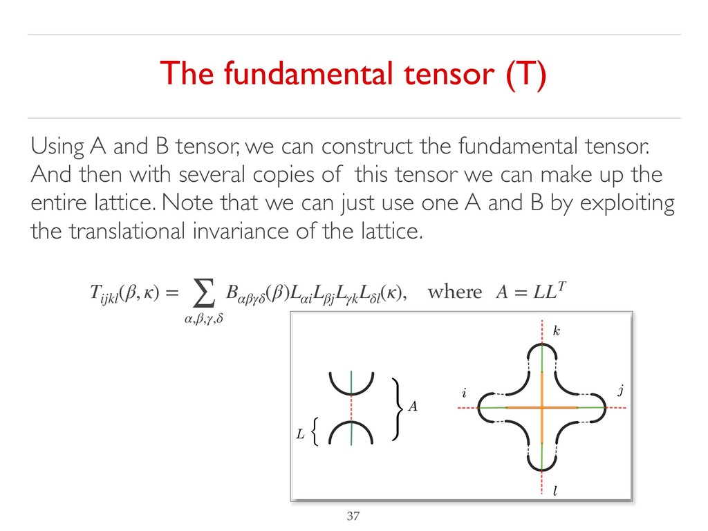
37. !37 The fundamental tensor (T) Tijkl (β, κ) = ∑ α,β,γ,δ Bαβγδ (β)Lαi Lβj Lγk Lδl (κ), where A = LLT Using A and B tensor, we can construct the fundamental tensor. And then with several copies of this tensor we can make up the entire lattice. Note that we can just use one A and B by exploiting the translational invariance of the lattice.
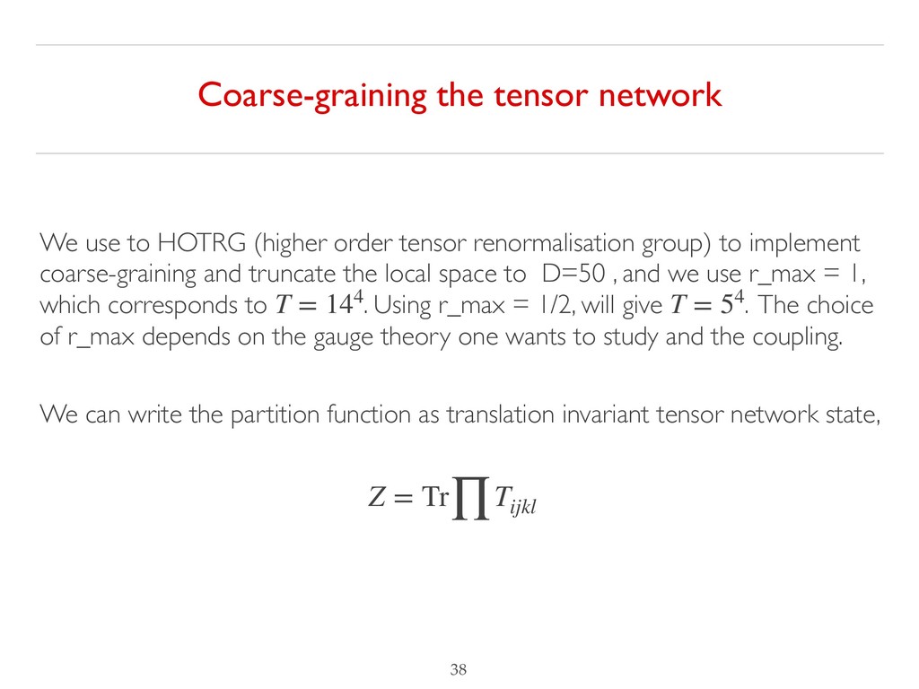
38. !38 Coarse-graining the tensor network We use to HOTRG (higher order tensor renormalisation group) to implement coarse-graining and truncate the local space to D=50 , and we use r_max = 1, which corresponds to . Using r_max = 1/2, will give . The choice of r_max depends on the gauge theory one wants to study and the coupling. We can write the partition function as translation invariant tensor network state, T = 144 T = 54 Z = Tr∏Tijkl
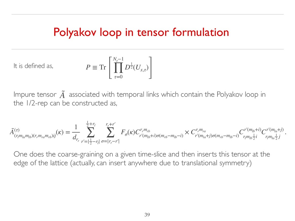
39. !39 Polyakov loop in tensor formulation P ≡ Tr [ Nτ −1 ∏ τ=0 D1 2(Ux,τ ) ] ˜ A ˜ A(τ) (rl mla mlb )(rr mra mrb )ij (κ) = 1 drr 1 2 +rl ∑ r′=|1 2 −rl | rr +r′ ∑ σ=|rr −r′| Fσ (κ)Crr mrb r′(mlb +i)σ(mrb −mlb −i) × Crr mra r′(mla +j)σ(mrb −mlb −i) Cr′(mlb +i) rl mlb 1 2 i Cr′(mla +j) rl mla 1 2 j . It is defined as, Impure tensor associated with temporal links which contain the Polyakov loop in the 1/2-rep can be constructed as, One does the coarse-graining on a given time-slice and then inserts this tensor at the edge of the lattice (actually, can insert anywhere due to translational symmetry)
40. !40 Exact results for β = 0 and κ = 0 For , we can write exact value of the Polyakov loop in terms of Bessel functions. This provides a simple check of the tensor formulation. β = 0
41. !41 Observables Matter susceptibility from tensor formulation compared with Monte Carlo results (about 1000 times slower). It is defined as, χκ = ∂2ln Z ∂κ2
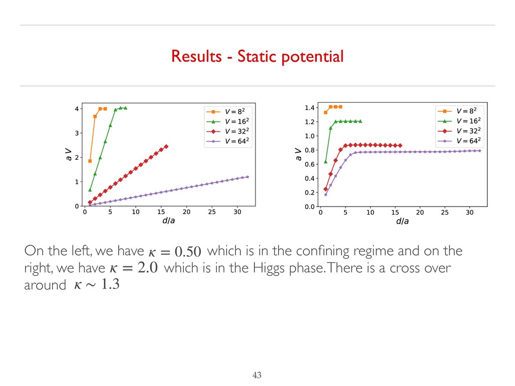
42. !42 Polyakov loop correlation - Confining & Higgs Phase In the limit of zero temperature, the correlator is given by, . This also provides a measure of monitoring confinement when (the slope gives , string tension). On the other hand, in a conformal theory, the potential is Coulomb such as N=4 SYM. In a Higgs phase, it is constant and independent of R. Two phases, 1) Confining phase, 2) Higgs-phase. C(R) = exp(−βV(R)) V ∝ R σ
43. !43 Results - Static potential κ = 0.50 κ = 2.0 κ ∼ 1.3 On the left, we have which is in the confining regime and on the right, we have which is in the Higgs phase. There is a cross over around
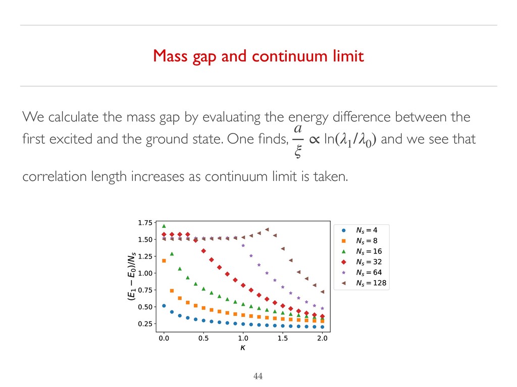
44. !44 We calculate the mass gap by evaluating the energy difference between the first excited and the ground state. One finds, and we see that correlation length increases as continuum limit is taken. a ξ ∝ ln(λ1 /λ0 ) Mass gap and continuum limit
45. !45 Conclusion Holography is crucial for understanding various aspects of quantum gravity. However, it is difficult to uncover all the features without exploring it at all scales & couplings. It is useful to turn to numerical methods and explore different approaches to understand it.
46. Thank you! !46