Recent results from lattice supersymmetry in 2 <= d < 4 dimensions

Transcript

1. Recent results from lattice supersymmetry in 2 ≤ d < 4 dimensions Raghav G. Jha Syracuse University arXiv: 1800.00012 and work in progress with Simon Catterall, Joel Giedt, Anosh Joseph, David Schaich & Toby Wiseman January 29, 2018 ICTS, Bangalore Raghav G. Jha Lattice simulations of SYM 1/24
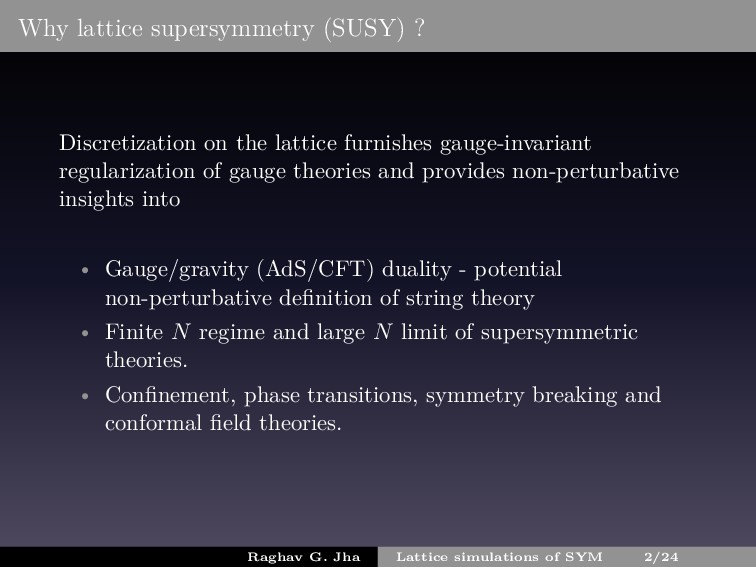
2. Why lattice supersymmetry (SUSY) ? Discretization on the lattice furnishes gauge-invariant regularization of gauge theories and provides non-perturbative insights into • Gauge/gravity (AdS/CFT) duality - potential non-perturbative definition of string theory • Finite N regime and large N limit of supersymmetric theories. • Confinement, phase transitions, symmetry breaking and conformal field theories. Raghav G. Jha Lattice simulations of SYM 2/24
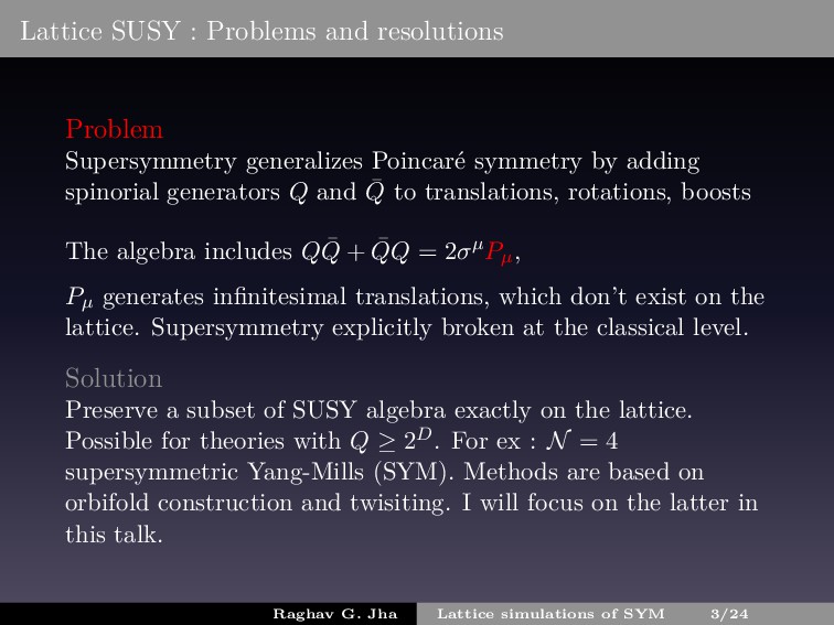
3. Lattice SUSY : Problems and resolutions Problem Supersymmetry generalizes Poincaré symmetry by adding spinorial generators Q and ¯ Q to translations, rotations, boosts The algebra includes Q ¯ Q + ¯ QQ = 2σµPµ, Pµ generates infinitesimal translations, which don’t exist on the lattice. Supersymmetry explicitly broken at the classical level. Solution Preserve a subset of SUSY algebra exactly on the lattice. Possible for theories with Q ≥ 2D. For ex : N = 4 supersymmetric Yang-Mills (SYM). Methods are based on orbifold construction and twisiting. I will focus on the latter in this talk. Raghav G. Jha Lattice simulations of SYM 3/24
4. Lattices in various dimensions THEORY R-SYMMETRY LATTICE CONSTRUCTION ? d = 2, Q = 4 SO(2) ⊗ U(1) ✓ d = 2, Q = 8 SO(4) ⊗ SU(2) ✓ d = 2, Q = 16 SO(8) ✓ d = 3, Q = 4 U(1)  d = 3, Q = 8 SO(3) ⊗ SU(2) ✓ d = 3, Q = 16 SO(7) ✓ d = 4, Q = 4 U(1)  d = 4, Q = 8 SO(2) ⊗ SU(2)  d = 4, Q = 16 SO(6) ✓ Raghav G. Jha Lattice simulations of SYM 4/24
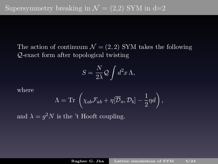
5. Supersymmetry breaking in N = (2,2) SYM in d=2 The action of continuum N = (2, 2) SYM takes the following Q-exact form after topological twisting S = N 2λ Q ∫ d2x Λ, where Λ = Tr ( χabFab + η[Da, Db] − 1 2 ηd ) , and λ = g2N is the ’t Hooft coupling. Raghav G. Jha Lattice simulations of SYM 5/24
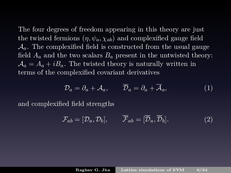
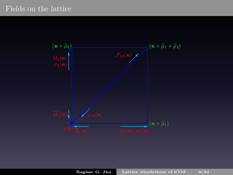
6. The four degrees of freedom appearing in this theory are just the twisted fermions (η, ψa, χab) and complexified gauge field Aa. The complexified field is constructed from the usual gauge field Aa and the two scalars Ba present in the untwisted theory: Aa = Aa + iBa. The twisted theory is naturally written in terms of the complexified covariant derivatives Da = ∂a + Aa, Da = ∂a + Aa, (1) and complexified field strengths Fab = [Da, Db], Fab = [Da, Db]. (2) Raghav G. Jha Lattice simulations of SYM 6/24
7. The nilpotent supersymmetry transformations associated with the scalar supercharge Q are given by Q Aa = ψa, Q ψa = 0, Q Aa = 0, Q χab = −Fab, Q η = d, Q d = 0. Raghav G. Jha Lattice simulations of SYM 7/24
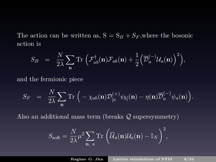
8. The action can be written as, S = SB + SF ,where the bosonic action is SB = N 2λ ∑ n Tr ( F† ab (n)Fab(n) + 1 2 ( D(−) a Ua(n) ) 2 ) , and the fermionic piece SF = N 2λ ∑ n Tr ( − χab(n)D(+) [a ψb] (n) − η(n)D(−) a ψa(n) ) . Also an additional mass term (breaks Q supersymmetry) Ssoft = N 2λ µ2 ∑ n, a Tr ( Ua(n)Ua(n) − IN ) 2 , Raghav G. Jha Lattice simulations of SYM 8/24
9. Fields on the lattice ✲ ✻ ✉ U1 (n) U1 (n), ψ1 (n) η(n) U2 (n) ψ2 (n) U2 (n) χ12 (n) F12 (n) (n + µ1 ) (n + µ1 + µ2 ) (n + µ2 ) ✒ ✠ ❄ ✻ ✲ ✛ Raghav G. Jha Lattice simulations of SYM 9/24
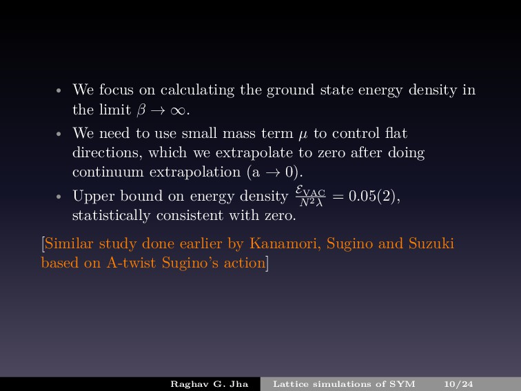
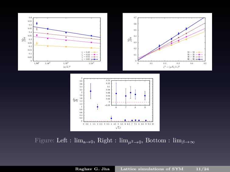
10. • We focus on calculating the ground state energy density in the limit β → ∞. • We need to use small mass term µ to control flat directions, which we extrapolate to zero after doing continuum extrapolation (a → 0). • Upper bound on energy density EVAC N2λ = 0.05(2), statistically consistent with zero. [Similar study done earlier by Kanamori, Sugino and Suzuki based on A-twist Sugino’s action] Raghav G. Jha Lattice simulations of SYM 10/24
11. 0 0.05 0.1 0.15 0.2 0.25 0.3 0.35 0.4 0.45 0.5 0.55 0.6 1/962 1/482 1/322 1/242 −S N2λ (a/L)2 ζ = 0.40 ζ = 0.50 ζ = 0.55 ζ = 0.60 0 0.1 0.2 0.3 0.4 0.5 0.6 0.7 0 0.1 0.2 0.3 0.4 0.5 −S N2λ ζ2 = (µNt /rτ )2 24 × 24 32 × 32 48 × 48 96 × 96 0 0.2 0.4 0.6 0.8 1 1.2 1.4 1.6 1.8 2 2.2 2.4 2.6 2.8 3 0 0.5 1 1.5 2 2.5 3 3.5 4 4.5 5 5.5 6 6.5 7 7.5 8 8.5 9 9.5 10 −0.02 0 0.02 0.04 0.06 0.08 0.1 0.12 0.14 6 7 8 9 EV AC N2λ √ λβ Figure: Left : lima→0 , Right : lim µ2→0 , Bottom : limβ→∞ Raghav G. Jha Lattice simulations of SYM 11/24
12. Applications to holography - gauge/gravity Original AdS/CFT correspondence 4D N = 4 U(N) super-Yang-Mills theory associated with N D3-branes, is dual to Type IIB string theory on AdS5 × S5 in the large N limit. More general holographic dualities in lower dimensions Maximally supersymmetric YM in p + 1 dimensions dual to Dp-branes At low temperatures, and in the decoupling limit : dual description in terms of black holes in Type II A/B supergravity Decoupling limit: N → ∞ and t = T/λ 1 3−p ≪ 1 Raghav G. Jha Lattice simulations of SYM 12/24
13. FIX HERE Show an example Raghav G. Jha Lattice simulations of SYM 13/24
14. Maximal SYM for p < 3 • Dimensionally reduce lattice N = 4 SYM along (3-p) spatial directions. • Dimensional reduction : A∗ 4 → A∗ p+1 giving a skewed torus with γ = −1/(p + 1) (γ = cosθ). • ’t Hooft coupling (λ) is dimensionful in p < 3 dimensions and we construct a dimensionless coupling given by ˆ λ = reff = λpβ3−p, where β = 1/T . • No phase transition (single de-confined phase) in 1-d QM case, richer structure for p = 1,2. Raghav G. Jha Lattice simulations of SYM 13/24
15. Regime of valid supergravity (SUGRA) description To have a valid SUGRA description, we need : • Radius of curvature should be large in units of α′. This implies rτ ≫ 1. • String coupling should be small. We can combine both requirements to get a constraint on the effective dimensionless coupling we can probe for a well-defined SUGRA description (p < 3) 1 ≪ λpβ3−p ≪ N 10−2p 7−p Raghav G. Jha Lattice simulations of SYM 14/24
16. History and dimensions • p=0 : [Hanada, Nishimura and Takeuchi in 0706.1647 + Catterall & Wiseman, 0706.3518] • p=1 : [See talk by David Schaich and Daisuke Kadoh] • p=2 : This talk [Preliminary work] • · · · · · · · · · • p = 3 : Thermodynamics of N = 4 SYM. Statement : Canwefindasmoothfunctionf(λ) ∋, f(0) = 1 and f(∞) = 3/4? Raghav G. Jha Lattice simulations of SYM 15/24
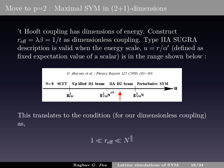
17. Move to p=2 : Maximal SYM in (2+1)-dimensions ’t Hooft coupling has dimensions of energy. Construct reff = λβ = 1/t as dimensionless coupling. Type IIA SUGRA description is valid when the energy scale, u = r/α′ (defined as fixed expectation value of a scalar) is in the range shown below : This translates to the condition (for our dimensionless coupling) as, 1 ≪ reff ≪ N 6 5 Raghav G. Jha Lattice simulations of SYM 16/24
18. Divergence of thermal partition function - I First discussed by [Kabat, Lifshitz and Lowe, hep-th/9910001, hep-th/0105171], the thermal partition function has divergence associated to ———– It was shown that the thermal Euclidean partition function can be schematically written as [Catterall & Wiseman, hep-th/0909.4947] , I ∼ kN log(g) + N2Ifinite So technically, one can avoid the issue of divergence if N → ∞ (another need for large N) because the finite contribution dominates. For the N we can access in our numerical simulations, we need to do more ! Use a mass term (µ) related to ζ in our lattice action to restrict the moduli space and then extract the finite piece carefully and compare to the thermodynamics of D0 branes. This divergence is supposed (??) to get milder with increasing p. Raghav G. Jha Lattice simulations of SYM 17/24
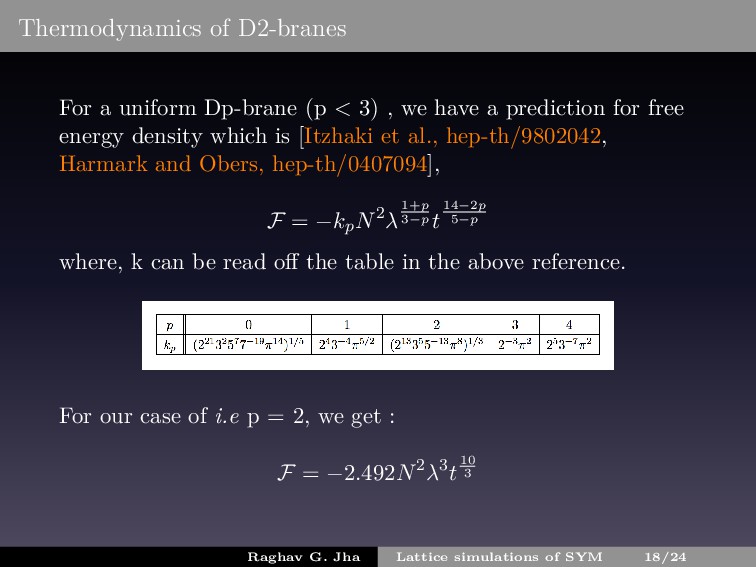
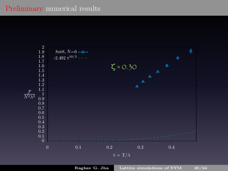
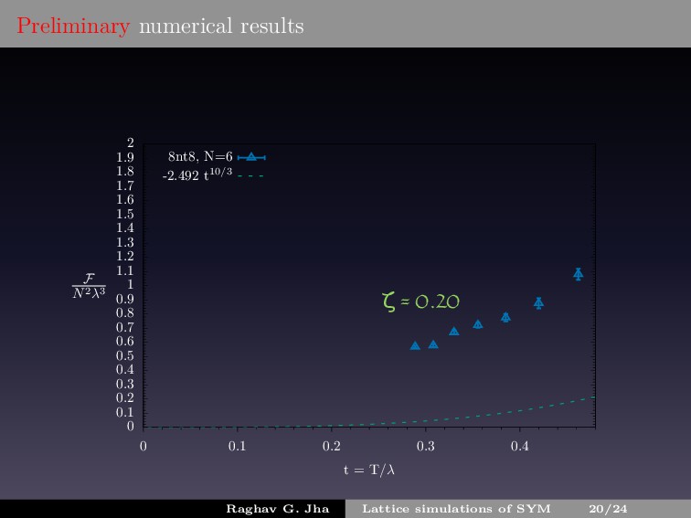
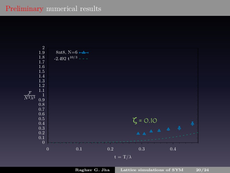
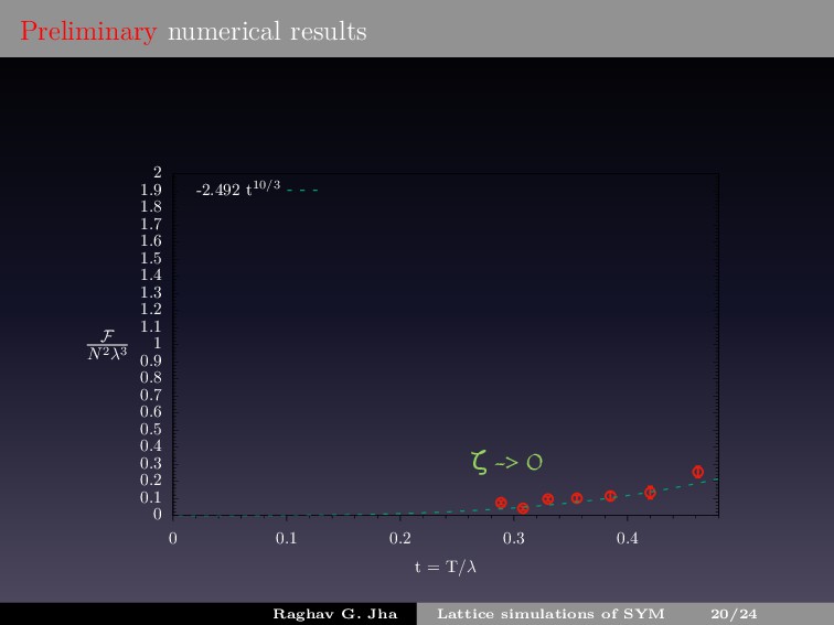
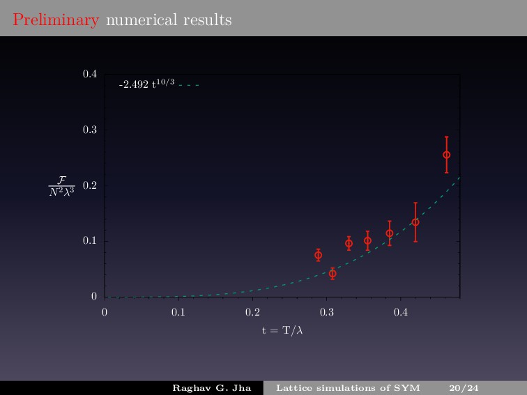
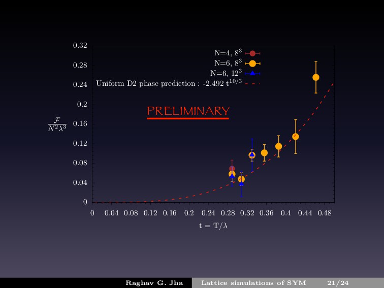
19. Thermodynamics of D2-branes For a uniform Dp-brane (p < 3) , we have a prediction for free energy density which is [Itzhaki et al., hep-th/9802042, Harmark and Obers, hep-th/0407094], F = −kpN2λ 1+p 3−p t 14−2p 5−p where, k can be read off the table in the above reference. For our case of i.e p = 2, we get : F = −2.492N2λ3t10 3 Raghav G. Jha Lattice simulations of SYM 18/24
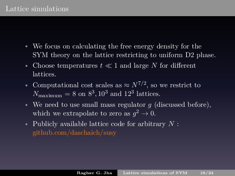
20. Lattice simulations • We focus on calculating the free energy density for the SYM theory on the lattice restricting to uniform D2 phase. • Choose temperatures t ≪ 1 and large N for different lattices. • Computational cost scales as ≈ N7/2, so we restrict to Nmaximum = 8 on 83, 103 and 123 lattices. • We need to use small mass regulator g (discussed before), which we extrapolate to zero as g2 → 0. • Publicly available lattice code for arbitrary N : github.com/daschaich/susy Raghav G. Jha Lattice simulations of SYM 19/24
21. Preliminary numerical results 0 0.1 0.2 0.3 0.4 0.5 0.6 0.7 0.8 0.9 1 1.1 1.2 1.3 1.4 1.5 1.6 1.7 1.8 1.9 2 0 0.1 0.2 0.3 0.4 F N2 3 t = T/ 8nt8, N=6 -2.492 t10/3 ζ = 0.30 Raghav G. Jha Lattice simulations of SYM 20/24
22. Preliminary numerical results 0 0.1 0.2 0.3 0.4 0.5 0.6 0.7 0.8 0.9 1 1.1 1.2 1.3 1.4 1.5 1.6 1.7 1.8 1.9 2 0 0.1 0.2 0.3 0.4 F N2 3 t = T/ 8nt8, N=6 -2.492 t10/3 ζ = 0.20 Raghav G. Jha Lattice simulations of SYM 20/24
23. Preliminary numerical results 0 0.1 0.2 0.3 0.4 0.5 0.6 0.7 0.8 0.9 1 1.1 1.2 1.3 1.4 1.5 1.6 1.7 1.8 1.9 2 0 0.1 0.2 0.3 0.4 F N2 3 t = T/ 8nt8, N=6 -2.492 t10/3 ζ = 0.10 Raghav G. Jha Lattice simulations of SYM 20/24
24. Preliminary numerical results 0 0.1 0.2 0.3 0.4 0.5 0.6 0.7 0.8 0.9 1 1.1 1.2 1.3 1.4 1.5 1.6 1.7 1.8 1.9 2 0 0.1 0.2 0.3 0.4 F N2 3 t = T/ -2.492 t10/3 ζ -> 0 Raghav G. Jha Lattice simulations of SYM 20/24
25. Preliminary numerical results 0 0.1 0.2 0.3 0.4 0 0.1 0.2 0.3 0.4 F N2λ3 t = T/λ -2.492 t10/3 Raghav G. Jha Lattice simulations of SYM 20/24
26. 0 0.04 0.08 0.12 0.16 0.2 0.24 0.28 0.32 0 0.04 0.08 0.12 0.16 0.2 0.24 0.28 0.32 0.36 0.4 0.44 0.48 F N2 3 t = T/ N=4, 83 N=6, 83 N=6, 123 Uniform D2 phase prediction : -2.492 t10/3 PRELIMINARY Raghav G. Jha Lattice simulations of SYM 21/24
27. Wilson loops in 3d-maximal SYM theory The quark-anti-quark potential calculated for this theory goes as [Maldacena, hep-th/9803002] E ∼ (g2 Y M N)1/3 L2/3 ∼ (αrτ )1/3 L This is only valid for αλβ ≫ 1, choosing α ∼ O(1) implies that λβ ≫ 1. Calculated only when the size of the loop is big [not perturbative] ! Raghav G. Jha Lattice simulations of SYM 22/24
28. Go back Raghav G. Jha Lattice simulations of SYM 23/24
29. Thank you ! Raghav G. Jha Lattice simulations of SYM 24/24
30. Thank you ! Funding and computing resources Raghav G. Jha Lattice simulations of SYM 24/24
31. Backup 1 Lower-dimensional sixteen supercharge SYM with apbc has no sign problem. Raghav G. Jha Lattice simulations of SYM 24/24
32. Backup 2 β L A B O L2 L2 D1L2 (L1 ) D1L2 (β) TrU = 0 TrV = 0 TrU = 0 TrV = 0 TrW = 0 TrU = 0 TrV = 0 TrW = 0 TrU = 0 TrV = 0 TrW = 0 D2L2 (β,L1 ) TrW = 0 C gravity D ? D0L2 Raghav G. Jha Lattice simulations of SYM 24/24
33. Backup – Raghav G. Jha Lattice simulations of SYM 24/24
34. Backup – Raghav G. Jha Lattice simulations of SYM 24/24
35. Backup – Raghav G. Jha Lattice simulations of SYM 24/24
36. Backup – Raghav G. Jha Lattice simulations of SYM 24/24