A novel method to retrieve AOT from high-resolution optical satellite images using an extended version of the Haze Optimised Transform

Transcript

1. 1 A novel method to retrieve AOT from high-resolution optical satellite images using an extended version of the Haze Optimized Transform Robin Wilson, Edward Milton & Joanna Nield r.t.wilson@soton.ac.uk @sciremotesense
2. MODIS 10km MAIAC 1km
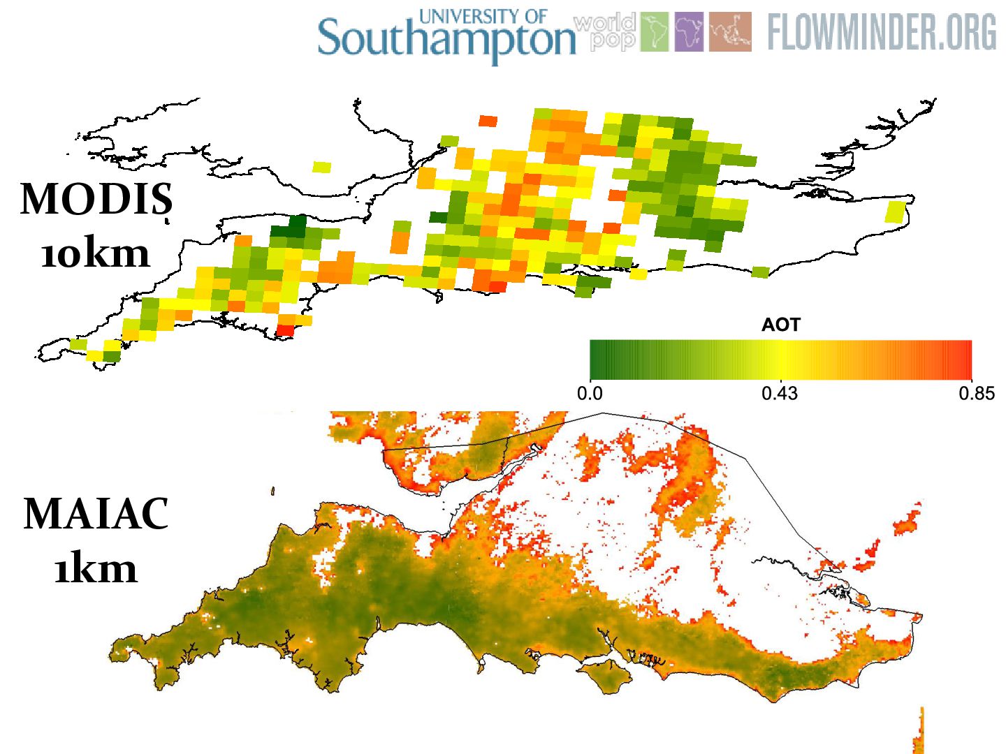
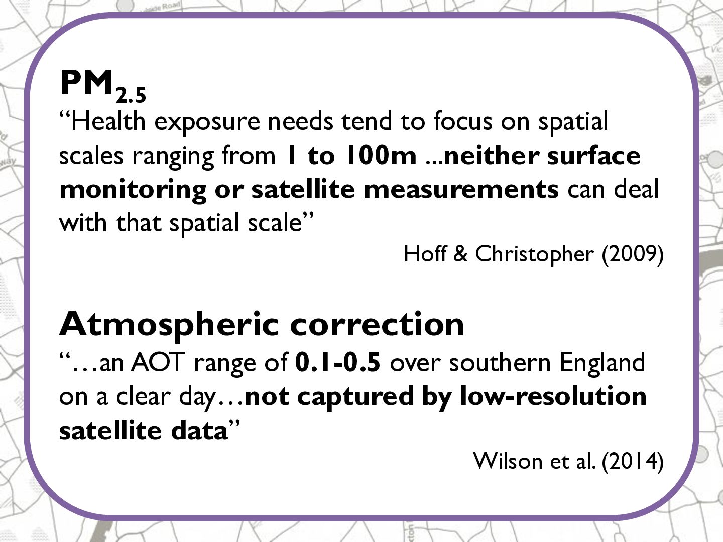
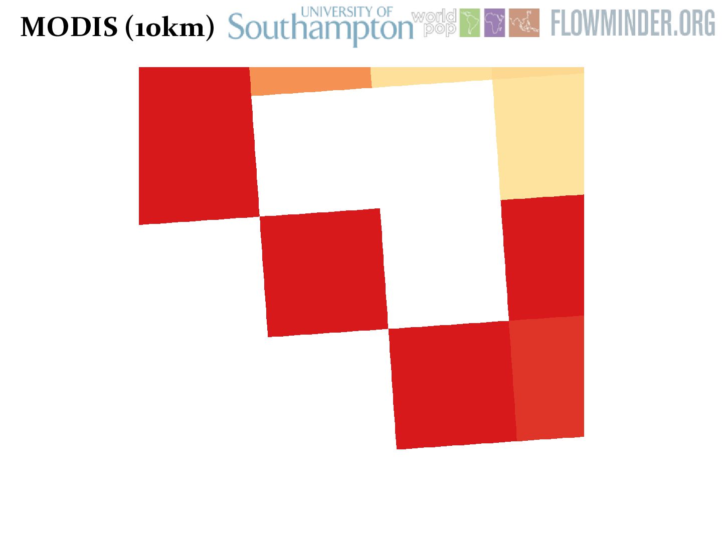
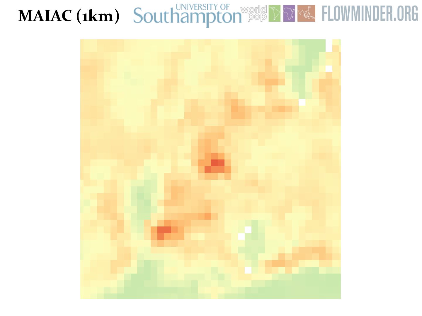
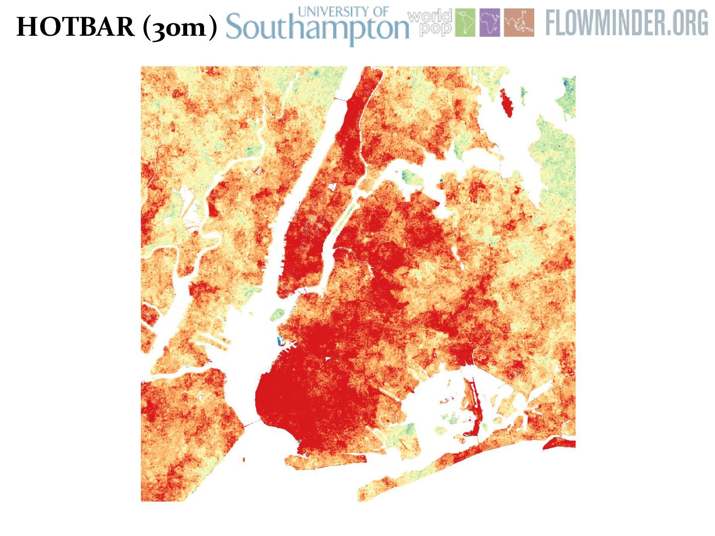
3. PM2.5 “Health exposure needs tend to focus on spatial scales ranging from 1 to 100m ...neither surface monitoring or satellite measurements can deal with that spatial scale” Hoff & Christopher (2009) Atmospheric correction “…an AOT range of 0.1-0.5 over southern England on a clear day…not captured by low-resolution satellite data” Wilson et al. (2014)
4. 4 Radiative Transfer Aerosols cause scattering Path Radiance Ground Radiance Adjacent Radiance But, we measure the sum!
5. 5 Radiative Transfer Aerosols cause scattering Path Radiance Ground Radiance Adjacent Radiance But, we measure the sum! How do we separate these? Polarisation, Multi-temporal, Multi-angle…
6. Haze Optimized Transform (HOT) Blue Red Haze = Aerosols Zhang et al. (2002) Distance ∝ Haze
7. HOTBAR Haze Optimised Transform based Aerosol Retrieval 1. Input: Landsat image 2. Estimate the Clear Line 3. Correct for land-cover effects 4. Link HOT values to AOT 5. Output: AOT image 7
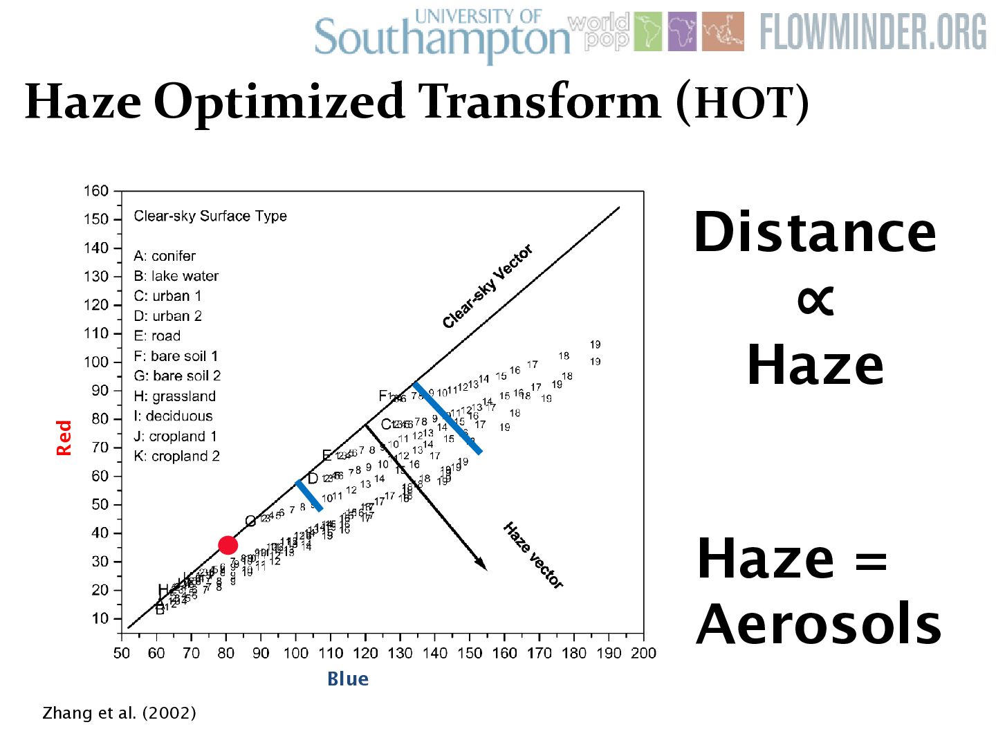
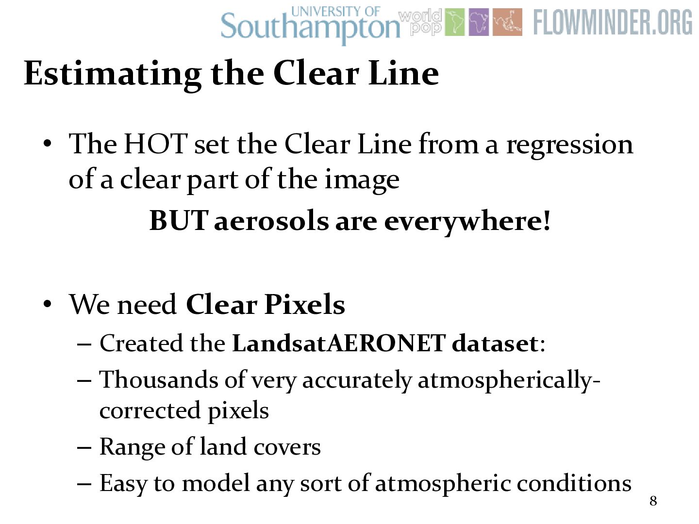
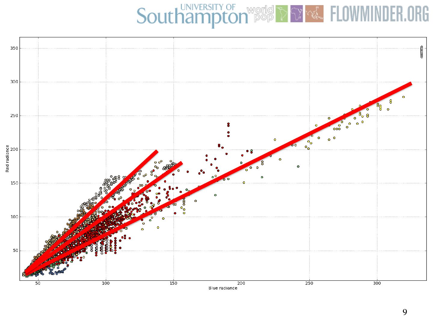
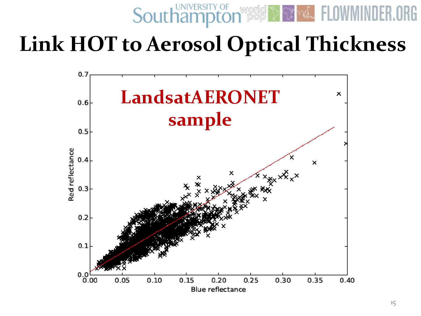
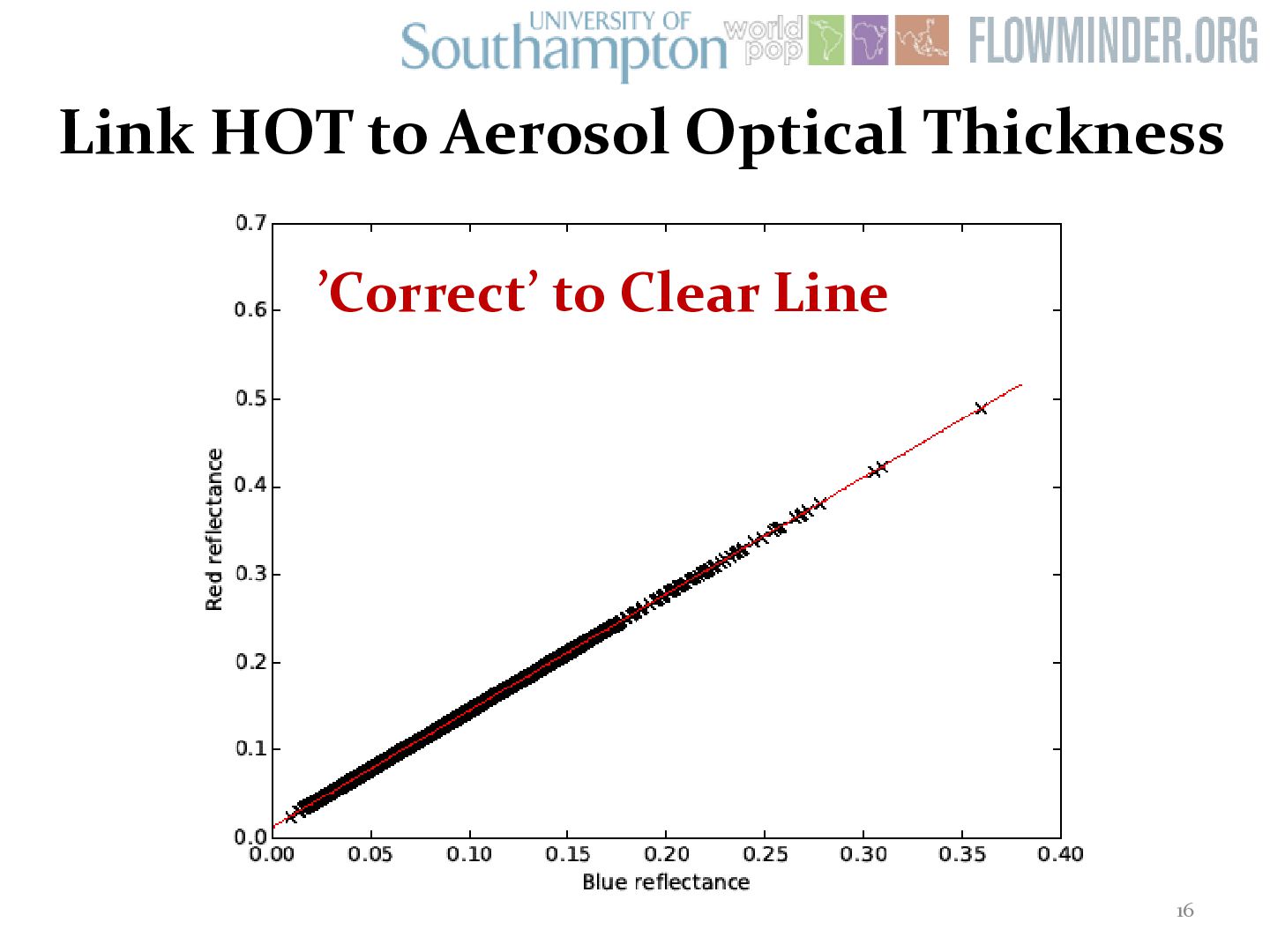
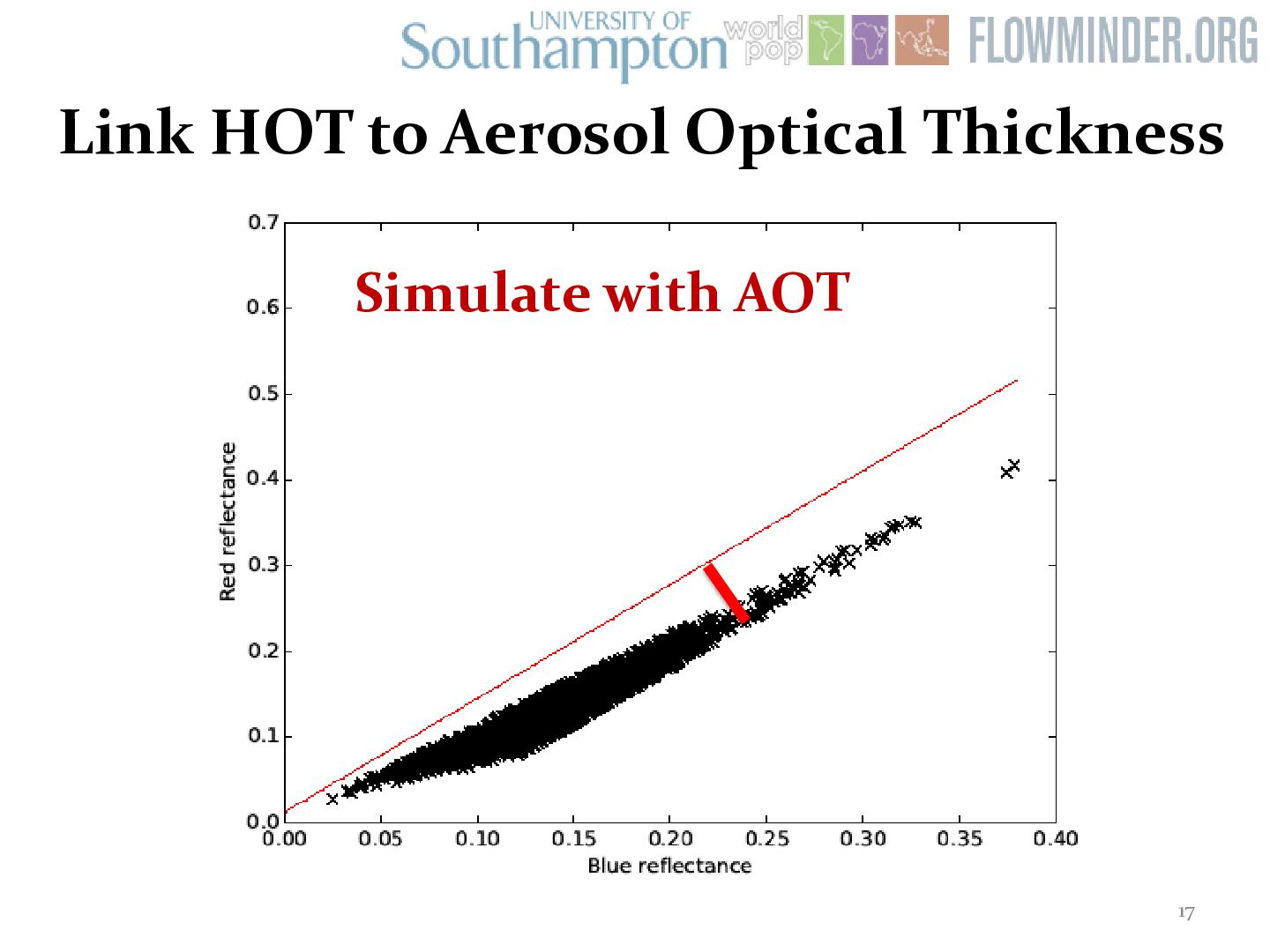
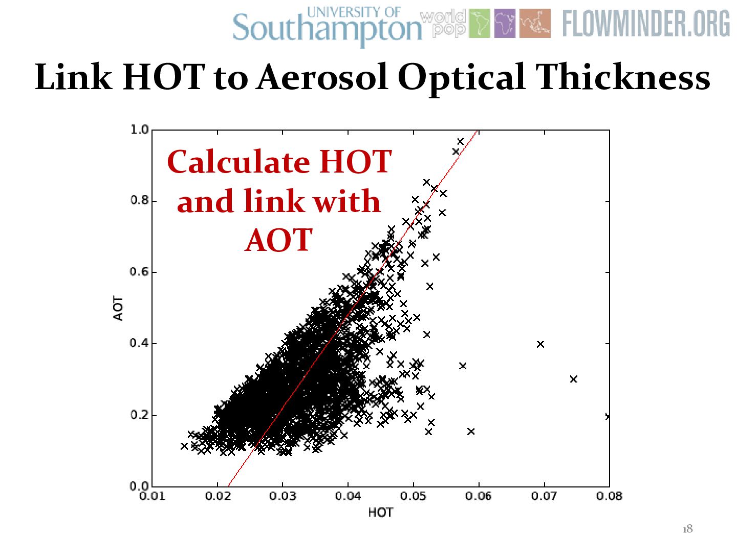
8. Estimating the Clear Line • The HOT set the Clear Line from a regression of a clear part of the image BUT aerosols are everywhere! • We need Clear Pixels – Created the LandsatAERONET dataset: – Thousands of very accurately atmospherically- corrected pixels – Range of land covers – Easy to model any sort of atmospheric conditions 8
10. Monte Carlo Regression • Clear Line depends on land cover • So, get land cover proportions (from GlobCover) • Estimate Clear Line from the LandsatAERONET dataset with a Monte Carlo Regression process 10
11. Correcting for Land Cover effects 11
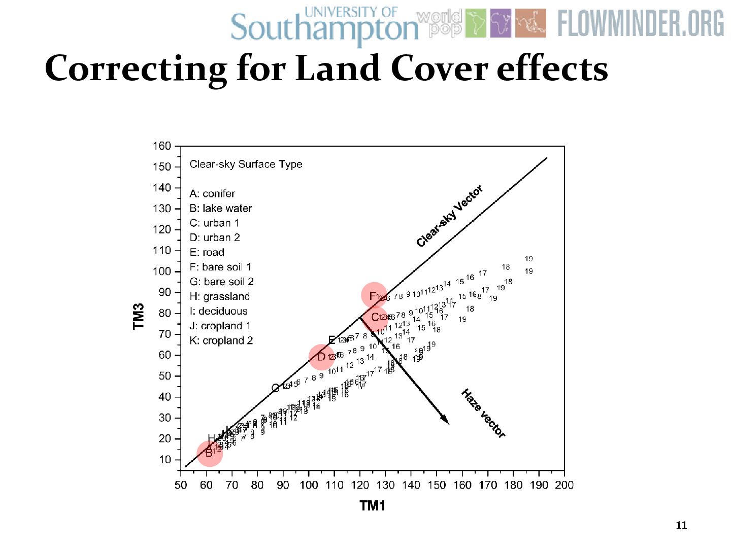
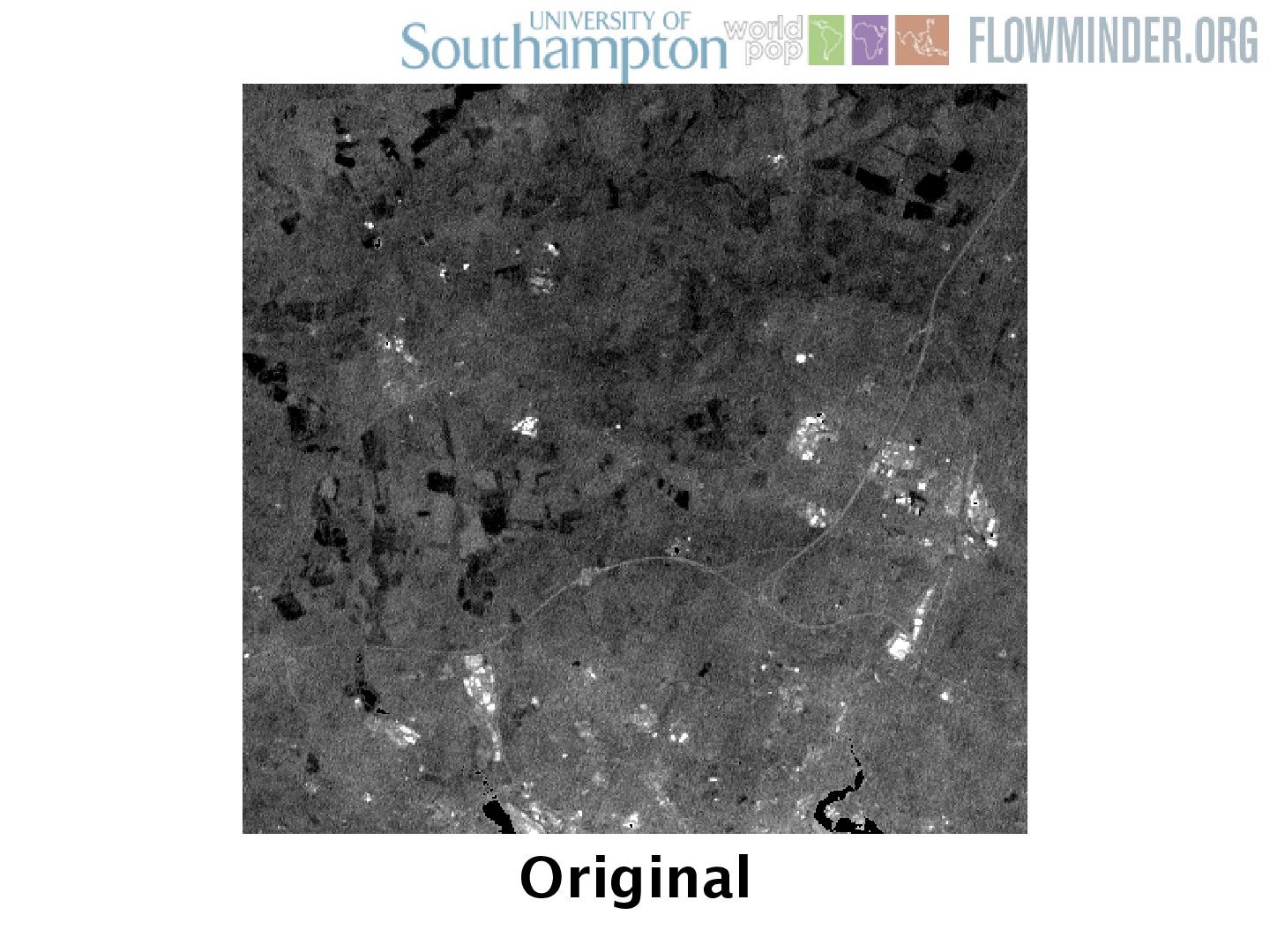
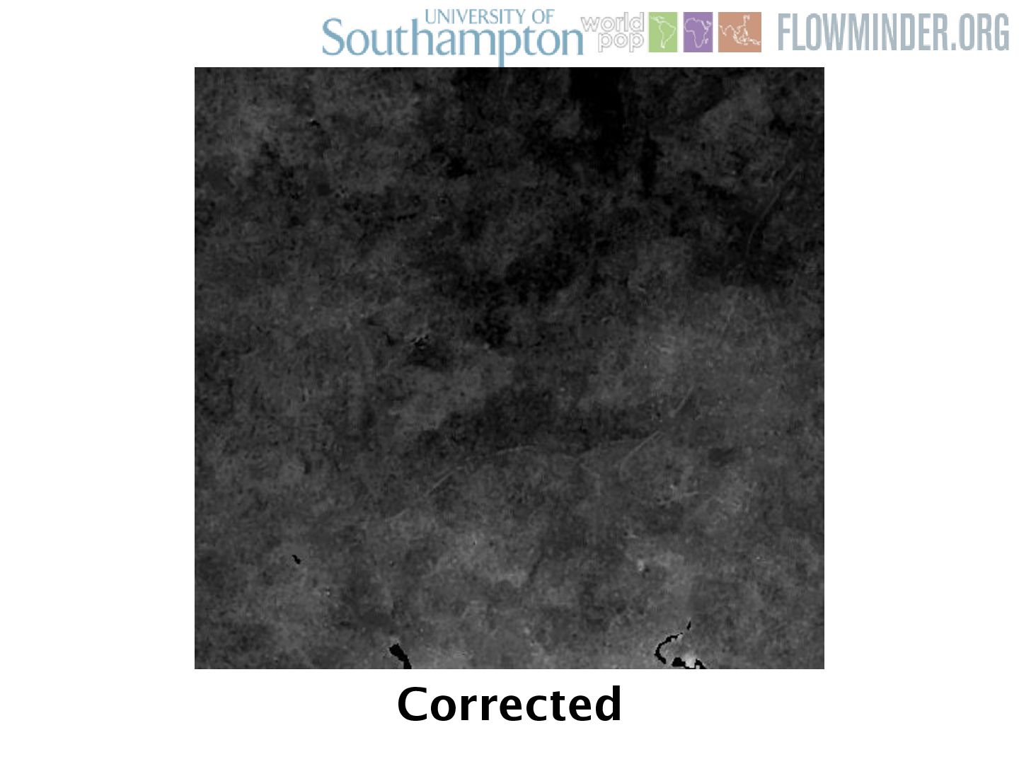
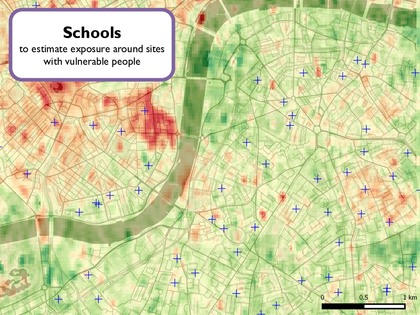
12. Correcting for Land Cover effects • The HOT is not Land Cover invariant • We need to correct for this – how? – Aerosols mix in the atmosphere → no sharp boundaries – Land covers often have sharp boundaries • Look for sharp boundaries, correct the pixel values inside these ‘objects’ → Object-based Image Analysis 12
13. Original
14. Corrected
15. Link HOT to Aerosol Optical Thickness 15 LandsatAERONET sample
16. 16 Link HOT to Aerosol Optical Thickness ’Correct’ to Clear Line
17. 17 Link HOT to Aerosol Optical Thickness Simulate with AOT
18. 18 Link HOT to Aerosol Optical Thickness Calculate HOT and link with AOT
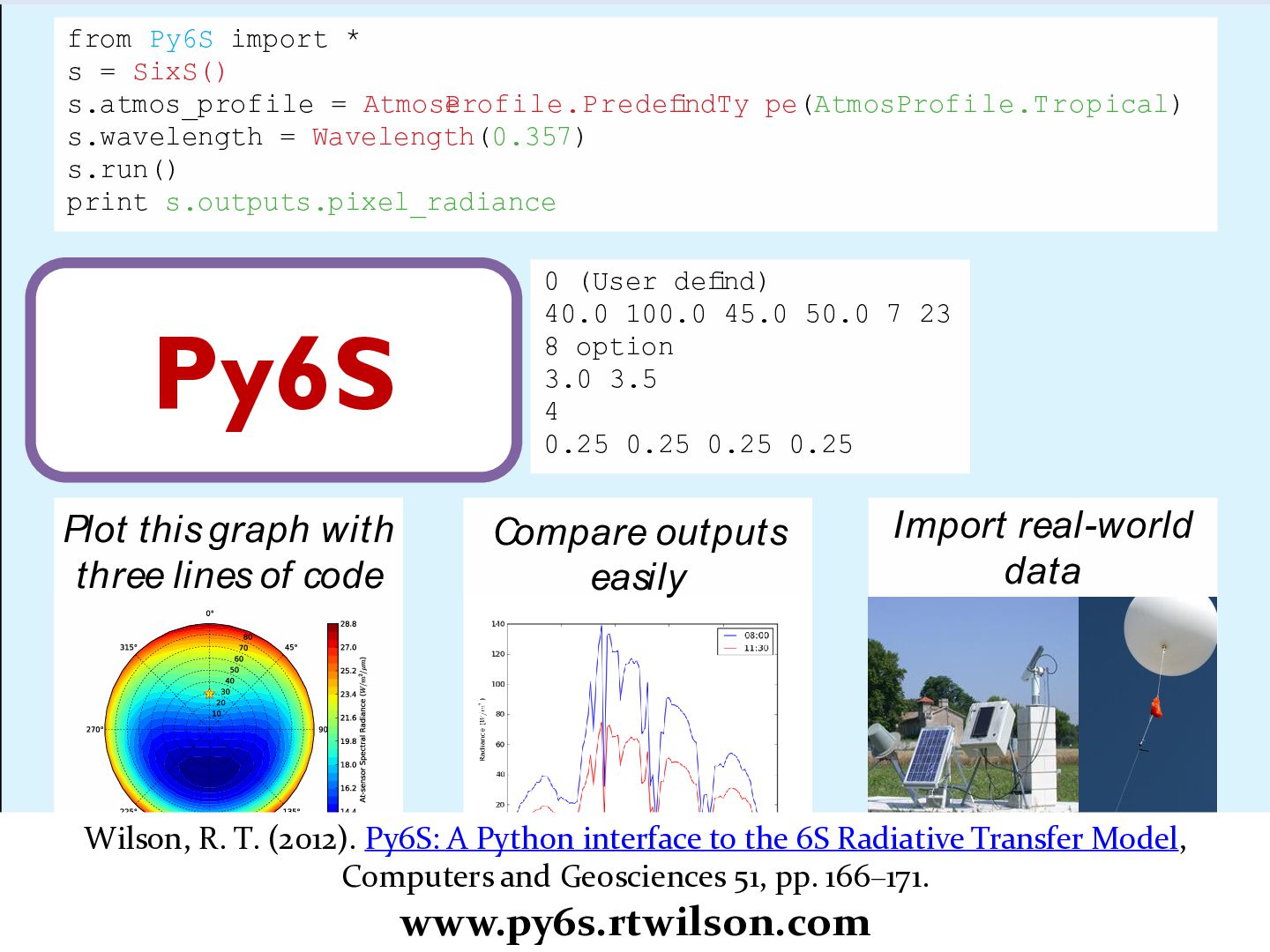
19. 19 0 (User def i nd) 40.0 100.0 45.0 50.0 7 23 8 option 3.0 3.5 4 0.25 0.25 0.25 0.25 from Py6S import * s = SixS() s.atmos_profile = AtmosProfile.Predef i n e dTy pe(AtmosProfile.Tropical) s.wavelength = Wavelength(0.357) s.run() print s.outputs.pixel_radiance Instead of this: Plot this graph with three lines of code Compare outputs easily Import real-world data Wilson, R. T., Py6S: A Python interface to the 6S Radiative Transfer Model Computers and Geosciences, Accepted Manuscript Wilson, R. T. (2012). Py6S: A Python interface to the 6S Radiative Transfer Model, Computers and Geosciences 51, pp. 166–171. www.py6s.rtwilson.com Py6S
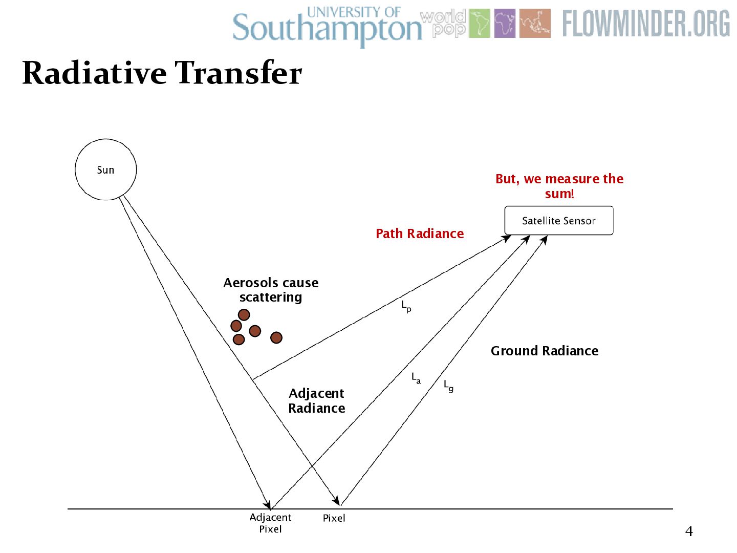
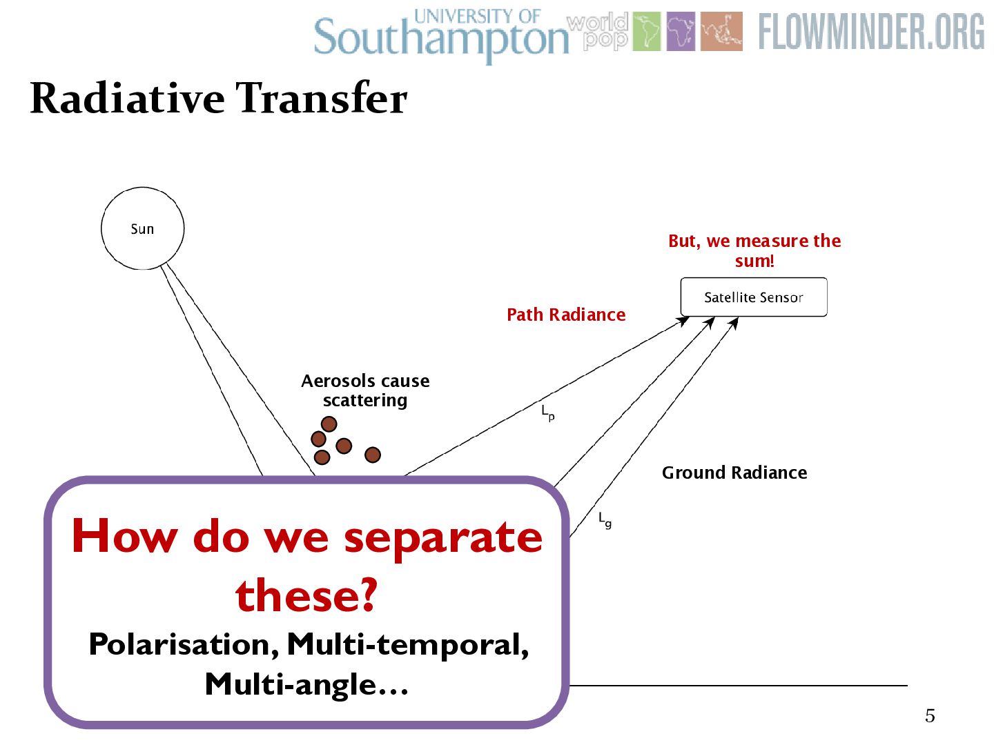
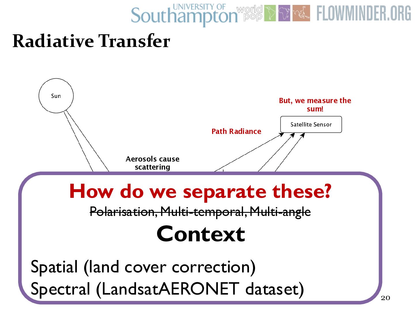
20. 20 Radiative Transfer Aerosols cause scattering Path Radiance Ground Radiance Adjacent Radiance But, we measure the sum! How do we separate these? Polarisation, Multi-temporal, Multi-angle Context Spatial (land cover correction) Spectral (LandsatAERONET dataset)
21. MODIS (10km)
22. MAIAC (1km)
23. HOTBAR (30m)
24. Validation shows robust performance MODIS 10km data: 60% within ± 0.13 OMI 15km data: RMSE = 0.15 Error comparable to other methods, but at 100,000 times the resolution of the MODIS 10km product
25. True per-pixel atmospheric correction
26. Landsat B1 Blue Landsat B2 Green Error compared with ground spectral measurements
27. PM2.5 concentrations Estimated from AOT using van Donkelaar et al. (2010) conversion factors
29. Schools to estimate exposure around sites with vulnerable people
30. • Ongoing production of a global product, in association with • Includes extension to Landsat 8 & operationalisation • Applications • PM2.5 mapping for exposure estimation • True per-pixel atmospheric correction • and more… Ongoing work
31. 31 Any questions? r.t.wilson@soton.ac.uk @sciremotesense