XArray: the power of pandas for multi-dimensional arrays

Transcript

1. XArray: the power of pandas for multidimensional arrays Robin Wilson @sciremotesense robin@rtwilson.com Slides: Code: http://xarray.pydata.org http://bit.do/xarray_pyconuk https://github.com/robintw/XArray_PyConUK2018
2. Satellite air quality data (from the MODIS MAIAC product)
3. Problem
4. Problem We have many decades of daily raster data, and want to get:
5. Problem We have many decades of daily raster data, and want to get: Seasonal means and standard deviations
6. Problem We have many decades of daily raster data, and want to get: Seasonal means and standard deviations Long time-series across specific points
7. Problem We have many decades of daily raster data, and want to get: Seasonal means and standard deviations Long time-series across specific points Individual images at specific times
8. The 'simple' solution
9. The 'simple' solution Load in the image data (using GDAL or rasterio)
10. The 'simple' solution Load in the image data (using GDAL or rasterio) Store in a large 3D numpy array (dimensions: X, Y and time)
11. The 'simple' solution Load in the image data (using GDAL or rasterio) Store in a large 3D numpy array (dimensions: X, Y and time) Index, slice and dice the array...
12. The 'simple' solution Load in the image data (using GDAL or rasterio) Store in a large 3D numpy array (dimensions: X, Y and time) Index, slice and dice the array... Not as easy it sounds...need to keep track of everything!
13. Enter XArray The power of pandas for multidimensional arrays
14. In [2]: import xarray as xr
15. Quick example In [3]: PM25 = xr.open_dataarray('/Users/robin/code/MAIACProcessing/All2014.nc')
16. Quick example In [3]: In [4]: PM25 = xr.open_dataarray('/Users/robin/code/MAIACProcessing/All2014.nc') PM25.shape Out[4]: (181, 1162, 1240)
17. Quick example In [3]: In [4]: In [5]: PM25 = xr.open_dataarray('/Users/robin/code/MAIACProcessing/All2014.nc') PM25.shape PM25.dims Out[4]: (181, 1162, 1240) Out[5]: ('time', 'y', 'x')
18. In [6]: seasonal = PM25.groupby('time.season').mean(dim='time')
19. In [6]: In [7]: seasonal = PM25.groupby('time.season').mean(dim='time') seasonal.plot.imshow(col='season', robust=True) Out[7]: <xarray.plot.facetgrid.FacetGrid at 0x30d4aceb8>
20. In [8]: time_series = PM25.isel(x=1000, y=1100).to_pandas().dropna()
21. In [8]: In [9]: time_series = PM25.isel(x=1000, y=1100).to_pandas().dropna() time_series Out[9]: time 2014-01-07 62.0 2014-01-17 121.0 2014-01-25 127.0 2014-02-10 135.0 2014-02-11 186.0 2014-02-18 237.0 2014-02-25 352.0 2014-02-26 293.0 2014-02-27 260.0 2014-03-01 165.0 2014-03-08 221.0 2014-03-09 221.0 2014-03-10 291.0 2014-03-13 552.0 2014-03-16 156.0 2014-03-21 159.0 2014-03-22 160.0 2014-03-23 163.0 2014-03-25 261.0 2014-03-30 362.0 2014-04-04 19.0 2014-04-09 19.0 2014-04-10 19.0 2014-04-11 19.0 2014-04-13 33.0 2014-04-14 19.0 2014-04-16 159.0 2014-04-18 53.0
22. In [10]: one_day = PM25.sel(time='2014-02-15')
23. In [10]: In [11]: one_day = PM25.sel(time='2014-02-15') one_day.plot(robust=True) Out[11]: <matplotlib.collections.QuadMesh at 0x31dcdeba8>
24. Summary In [12]: In [13]: In [14]: seasonal = PM25.groupby('time.season').mean(dim='time') time_series = PM25.isel(x=1000, y=1100).to_pandas().dropna() one_day = PM25.sel(time='2014-02-20')
25. Introduction to XArray
26. Introduction to XArray xarray.DataArray is a fancy, labelled version of a numpy.ndarray
27. Introduction to XArray xarray.DataArray is a fancy, labelled version of a numpy.ndarray xarray.Dataset is a collection of multiple DataArrays which share dimensions
28. Introduction to XArray xarray.DataArray is a fancy, labelled version of a numpy.ndarray xarray.Dataset is a collection of multiple DataArrays which share dimensions (A Dataset is a representation of a NetCDF file)
29. In [15]: arr = np.random.rand(3, 4, 2)
30. In [15]: In [16]: arr = np.random.rand(3, 4, 2) xr.DataArray(arr) Out[16]: <xarray.DataArray (dim_0: 3, dim_1: 4, dim_2: 2)> array([[[0.006194, 0.380531], [0.561032, 0.360739], [0.515117, 0.300988], [0.650297, 0.560798]], [[0.703038, 0.762046], [0.703794, 0.467468], [0.19292 , 0.395919], [0.344915, 0.874793]], [[0.570962, 0.881131], [0.758426, 0.582632], [0.419739, 0.634596], [0.720827, 0.12582 ]]]) Dimensions without coordinates: dim_0, dim_1, dim_2
31. In [17]: xr.DataArray(arr, dims=('x', 'y', 'time')) Out[17]: <xarray.DataArray (x: 3, y: 4, time: 2)> array([[[0.006194, 0.380531], [0.561032, 0.360739], [0.515117, 0.300988], [0.650297, 0.560798]], [[0.703038, 0.762046], [0.703794, 0.467468], [0.19292 , 0.395919], [0.344915, 0.874793]], [[0.570962, 0.881131], [0.758426, 0.582632], [0.419739, 0.634596], [0.720827, 0.12582 ]]]) Dimensions without coordinates: x, y, time
32. In [18]: da = xr.DataArray(arr, dims=('x', 'y', 'time'), coords={'x': [10, 20, 30], 'y': [0.3, 0.7, 1.3, 1.5], 'time': [datetime.datetime(2016, 3, 5), datetime.datetime(2016, 4, 7)]})
33. In [19]: da Out[19]: <xarray.DataArray (x: 3, y: 4, time: 2)> array([[[0.006194, 0.380531], [0.561032, 0.360739], [0.515117, 0.300988], [0.650297, 0.560798]], [[0.703038, 0.762046], [0.703794, 0.467468], [0.19292 , 0.395919], [0.344915, 0.874793]], [[0.570962, 0.881131], [0.758426, 0.582632], [0.419739, 0.634596], [0.720827, 0.12582 ]]]) Coordinates: * x (x) int64 10 20 30 * y (y) float64 0.3 0.7 1.3 1.5 * time (time) datetime64[ns] 2016-03-05 2016-04-07
34. In [20]: da.sel(time='2016-03-05') Out[20]: <xarray.DataArray (x: 3, y: 4)> array([[0.006194, 0.561032, 0.515117, 0.650297], [0.703038, 0.703794, 0.19292 , 0.344915], [0.570962, 0.758426, 0.419739, 0.720827]]) Coordinates: * x (x) int64 10 20 30 * y (y) float64 0.3 0.7 1.3 1.5 time datetime64[ns] 2016-03-05
35. In [21]: da.isel(time=1) Out[21]: <xarray.DataArray (x: 3, y: 4)> array([[0.380531, 0.360739, 0.300988, 0.560798], [0.762046, 0.467468, 0.395919, 0.874793], [0.881131, 0.582632, 0.634596, 0.12582 ]]) Coordinates: * x (x) int64 10 20 30 * y (y) float64 0.3 0.7 1.3 1.5 time datetime64[ns] 2016-04-07
36. In [22]: da.sel(x=slice(0, 20)) Out[22]: <xarray.DataArray (x: 2, y: 4, time: 2)> array([[[0.006194, 0.380531], [0.561032, 0.360739], [0.515117, 0.300988], [0.650297, 0.560798]], [[0.703038, 0.762046], [0.703794, 0.467468], [0.19292 , 0.395919], [0.344915, 0.874793]]]) Coordinates: * x (x) int64 10 20 * y (y) float64 0.3 0.7 1.3 1.5 * time (time) datetime64[ns] 2016-03-05 2016-04-07
37. In [23]: da.mean(dim='time') Out[23]: <xarray.DataArray (x: 3, y: 4)> array([[0.193362, 0.460886, 0.408053, 0.605548], [0.732542, 0.585631, 0.294419, 0.609854], [0.726047, 0.670529, 0.527168, 0.423323]]) Coordinates: * x (x) int64 10 20 30 * y (y) float64 0.3 0.7 1.3 1.5
38. In [24]: da.mean(dim=['x', 'y']) Out[24]: <xarray.DataArray (time: 2)> array([0.512272, 0.527288]) Coordinates: * time (time) datetime64[ns] 2016-03-05 2016-04-07
39. In [25]: PM25.sel(time='2014').groupby('time.month').std(dim='time') Out[25]: <xarray.DataArray 'data' (month: 6, y: 1162, x: 1240)> array([[[ nan, nan, ..., nan, nan], [ nan, nan, ..., nan, nan], ..., [ nan, nan, ..., nan, nan], [ nan, nan, ..., nan, nan]], [[ nan, nan, ..., nan, nan], [ 0. , nan, ..., nan, nan], ..., [ nan, nan, ..., nan, nan], [ nan, nan, ..., nan, nan]], ..., [[ 23.97684, 0. , ..., nan, nan], [ 1. , 2.5 , ..., nan, nan], ..., [ nan, nan, ..., nan, nan], [ nan, nan, ..., nan, nan]], [[146.48776, 125.04899, ..., nan, nan], [146.27904, 148.14934, ..., nan, nan], ..., [ nan, nan, ..., nan, nan], [ nan, nan, ..., nan, nan]]], dtype=float32) Coordinates: * y (y) float64 1.429e+06 1.428e+06 1.427e+06 1.426e+06 1.424e+06 ... * x (x) float64 -9.476e+05 -9.464e+05 -9.451e+05 -9.439e+05 ... * month (month) int64 1 2 3 4 5 6
40. Efficient processing with dask and dask.distributed
41. Efficient processing with dask and dask.distributed dask creates a computational graph of your processing steps, and then executes it as efficiently as possible.
42. Efficient processing with dask and dask.distributed dask creates a computational graph of your processing steps, and then executes it as efficiently as possible. This includes only loading data that is actually needed and only processing things once.
43. In [26]: data = xr.open_mfdataset(['DaskTest1.nc', 'DaskTest2.nc'], chunks={'time':10}) ['data'] avg = data.mean(dim='time') Dask execution graph
44. In [27]: seasonal = data.groupby('time.season').mean(dim='time') Dask execution graph
45. dask.distributed All of these different chunks, and separate processing chains can be run on separate processes or separate computers.
46. Getting data into xarray
47. Getting data into xarray xarray can read various formats directly: NetCDF HDF GRIB
48. Getting data into xarray xarray can read various formats directly: NetCDF HDF GRIB xarray can now use rasterio to read loads of geographic raster formats
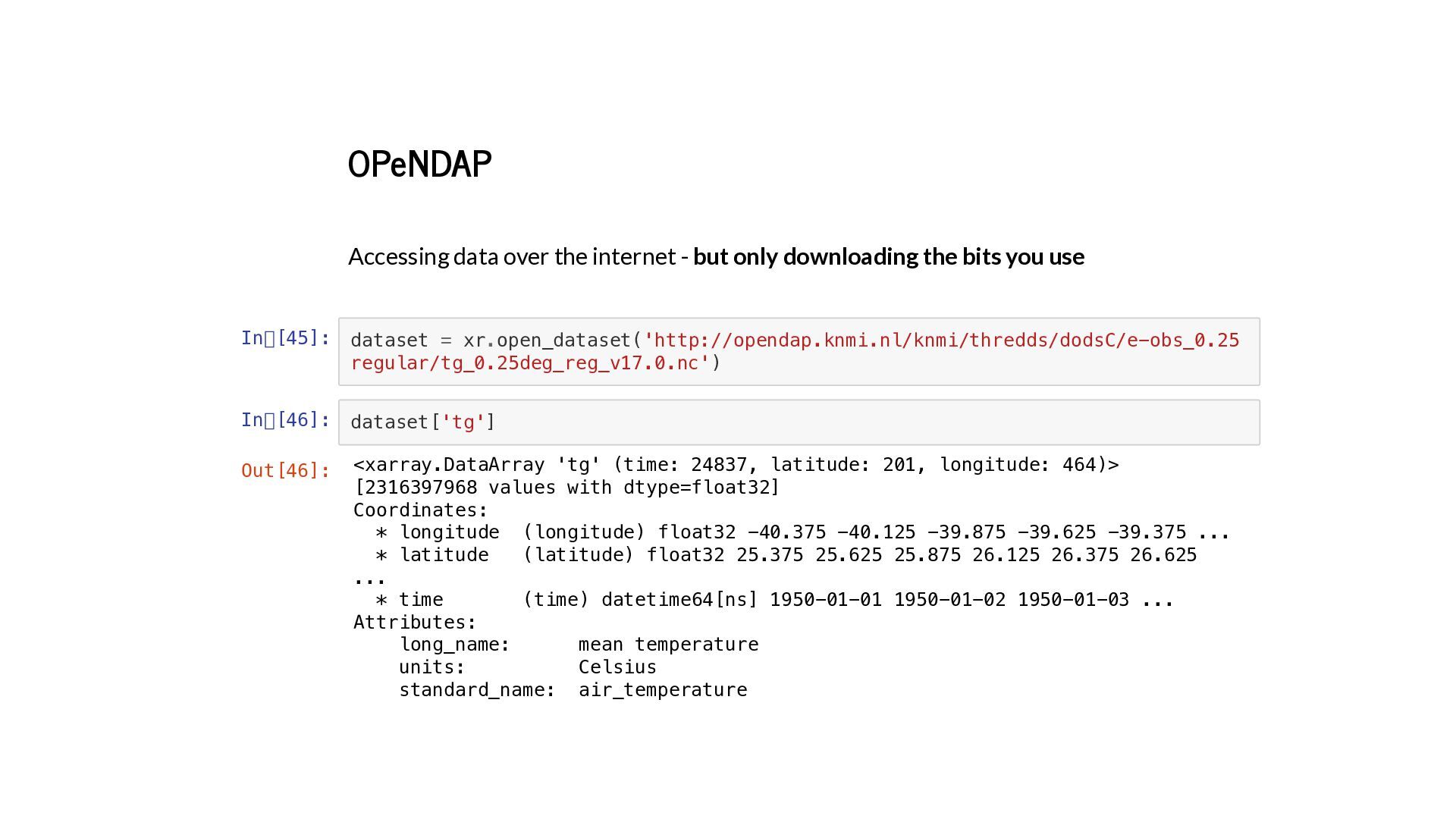
49. In [28]: xr.open_rasterio('satellite_image.tif') Out[28]: <xarray.DataArray (band: 3, y: 1644, x: 1435)> [7077420 values with dtype=uint8] Coordinates: * band (band) int64 1 2 3 * y (y) float64 1.484e+05 1.484e+05 1.484e+05 1.484e+05 1.484e+05 ... * x (x) float64 4.301e+05 4.301e+05 4.302e+05 4.302e+05 4.302e+05 ... Attributes: transform: (10.0, 0.0, 430130.2396, 0.0, -10.0, 148415.8755, 0.0, 0.0, ... crs: +ellps=airy +k=0.999601 +lat_0=49 +lon_0=-2 +no_defs +proj= t... res: (10.0, 10.0) is_tiled: 0 nodatavals: (nan, nan, nan)
50. Example - combining multiple satellite data files into a time- series
51. Example - combining multiple satellite data files into a time- series Take a large number of files, one from each orbit of a satellite, and put them into one large array with a time dimension.
52. Example - combining multiple satellite data files into a time- series Take a large number of files, one from each orbit of a satellite, and put them into one large array with a time dimension. In [30]: def file_to_da(filename): da = xr.open_rasterio(filename) time_str = os.path.basename(filename)[17:-17] time_obj = datetime.datetime.strptime(time_str, '%Y%j%H%M') da.coords['time'] = time_obj return da.isel(band=0)
53. Example - combining multiple satellite data files into a time- series Take a large number of files, one from each orbit of a satellite, and put them into one large array with a time dimension. In [30]: In [32]: def file_to_da(filename): da = xr.open_rasterio(filename) time_str = os.path.basename(filename)[17:-17] time_obj = datetime.datetime.strptime(time_str, '%Y%j%H%M') da.coords['time'] = time_obj return da.isel(band=0) list_of_data_arrays = [file_to_da(filename) for filename in files]
54. Example - combining multiple satellite data files into a time- series Take a large number of files, one from each orbit of a satellite, and put them into one large array with a time dimension. In [30]: In [32]: In [33]: def file_to_da(filename): da = xr.open_rasterio(filename) time_str = os.path.basename(filename)[17:-17] time_obj = datetime.datetime.strptime(time_str, '%Y%j%H%M') da.coords['time'] = time_obj return da.isel(band=0) list_of_data_arrays = [file_to_da(filename) for filename in files] combined = xr.concat(list_of_data_arrays, dim='time')
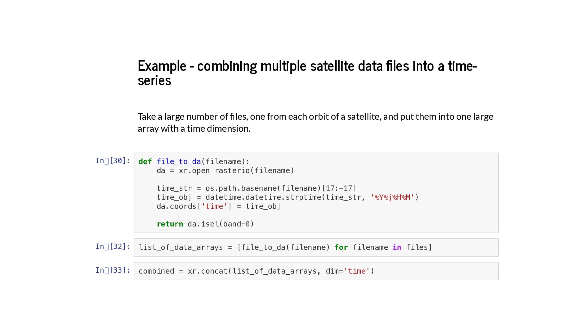
55. In [34]: In [35]: combined.shape combined.coords Out[34]: (10, 1162, 1240) Out[35]: Coordinates: band int64 1 * y (y) float64 1.429e+06 1.427e+06 1.426e+06 1.425e+06 1.424e+06 ... * x (x) float64 -9.47e+05 -9.458e+05 -9.445e+05 -9.432e+05 ... * time (time) datetime64[ns] 2003-04-16T14:40:00 2002-03-19T11:20:00 ...
56. Getting raster data out of xarray In [38]: In [39]: In [41]: from xarray_to_rasterio import xarray_to_rasterio mean = combined.mean(dim='time', keep_attrs=True) xarray_to_rasterio(mean, 'Mean.tif')
57. A few tasters...
58. Interpolation In [69]: In [70]: PM25.interp(x=318193.5, y=176849.7).to_pandas().dropna().head() PM25.interp(x=318193.5, y=176849.7, method='nearest').to_pandas().dropna().head () Out[69]: time 2014-01-07 74.390257 2014-01-09 42.588762 2014-01-19 84.464250 2014-02-07 37.803606 2014-02-11 67.395553 dtype: float64 Out[70]: time 2014-01-07 72.0 2014-01-09 42.0 2014-01-19 82.0 2014-01-27 159.0 2014-02-01 297.0 dtype: float32
59. Resampling time series In [55]: PM25.resample(time='1M').mean(dim='time') Out[55]: <xarray.DataArray 'data' (time: 6, y: 1162, x: 1240)> array([[[ nan, nan, ..., nan, nan], [ nan, nan, ..., nan, nan], ..., [ nan, nan, ..., nan, nan], [ nan, nan, ..., nan, nan]], [[ nan, nan, ..., nan, nan], [ 20. , nan, ..., nan, nan], ..., [ nan, nan, ..., nan, nan], [ nan, nan, ..., nan, nan]], ..., [[ 70.333336, 46. , ..., nan, nan], [ 49. , 53.5 , ..., nan, nan], ..., [ nan, nan, ..., nan, nan], [ nan, nan, ..., nan, nan]], [[333. , 326.5 , ..., nan, nan], [324.33334 , 334.33334 , ..., nan, nan], ..., [ nan, nan, ..., nan, nan], [ nan, nan, ..., nan, nan]]], dtype=float3 2)
60. Rolling windows In [71]: PM25.rolling(time=5).mean() Out[71]: <xarray.DataArray (time: 10, y: 1162, x: 1240)> array([[[nan, nan, ..., nan, nan], [nan, nan, ..., nan, nan], ..., [nan, nan, ..., nan, nan], [nan, nan, ..., nan, nan]], [[nan, nan, ..., nan, nan], [nan, nan, ..., nan, nan], ..., [nan, nan, ..., nan, nan], [nan, nan, ..., nan, nan]], ..., [[nan, nan, ..., nan, nan], [nan, nan, ..., nan, nan], ..., [nan, nan, ..., nan, nan], [nan, nan, ..., nan, nan]], [[nan, nan, ..., nan, nan], [nan, nan, ..., nan, nan], ..., [nan, nan, ..., nan, nan], [nan, nan, ..., nan, nan]]], dtype=float32) Coordinates:
61. OPeNDAP Accessing data over the internet - but only downloading the bits you use In [45]: In [46]: dataset = xr.open_dataset('http://opendap.knmi.nl/knmi/thredds/dodsC/e-obs_0.25 regular/tg_0.25deg_reg_v17.0.nc') dataset['tg'] Out[46]: <xarray.DataArray 'tg' (time: 24837, latitude: 201, longitude: 464)> [2316397968 values with dtype=float32] Coordinates: * longitude (longitude) float32 -40.375 -40.125 -39.875 -39.625 -39.375 ... * latitude (latitude) float32 25.375 25.625 25.875 26.125 26.375 26.625 ... * time (time) datetime64[ns] 1950-01-01 1950-01-02 1950-01-03 ... Attributes: long_name: mean temperature units: Celsius standard_name: air_temperature
62. In [47]: temperature = dataset['tg'] oneday = temperature.sel(time='2009-07-01') oneday.plot(robust=True) Out[47]: <matplotlib.collections.QuadMesh at 0x324b65080>
63. xarray extensions Simulation models in xarray (xarray-simlab) WRF Weather Forecasting Model functions (wrf-python) Empirical Orthogonal Functions (eofs) Many more at http://xarray.pydata.org/en/stable/faq.html#what-other-projects- leverage-xarray
64. In [48]: from eofs.xarray import Eof monthly = PM25.resample(time='M').mean('time') solver = Eof(monthly) results = solver.eofs()
65. In [49]: results.plot(col='mode', col_wrap=3, robust=True) Out[49]: <xarray.plot.facetgrid.FacetGrid at 0x324a77550>
66. Resources Slides: Code: XArray docs: robin@rtwilson.com @sciremotesense @robintw on Slack http://bit.do/xarray_pyconuk https://github.com/robintw/XArray_PyConUK2018 http://xarray.pydata.org/