Software Sustainability and Reproducible Research in Remote Sensing

Slides from a talk given at RSPSoc Wavelength 2013 in Glasgow, Scotland. In this talk I discuss the importance of Software Sustainability and Reproducible Research in Remote Sensing, and give a number of practical suggestions as to how to achieve it. It was presented as part of my Fellowship from the Software Sustainability Institute (www.software.ac.uk)

Transcript

1. Sustainable  So-ware  &   Reproducible  Research   in  Remote  Sensing     Robin  Wilson   Geography  and  Environment,  University  of  Southampton   &  So=ware  Sustainability  Ins@tute     www.rtwilson.com/academic     r.t.wilson@soton.ac.uk  @sciremotesense  
2. Discussion  Ques:ons         Not  just  Yes/No  –  but   why?      
3. Given  your  most  recent:   •  journal  ar@cle   •  conference  paper   •  presenta@on  at  this  conference   Could  I  reproduce  all  of  your   results,  from  the  raw  input   data  +  the  paper/thesis?  
4. Think  of  some  data  you’ve  collected  yourself…   Would  it  s:ll  be  useable  in  10   years  :me?  20  years?  30   years?  
5. If  you’ve  wriNen  scripts  or  code  of  any  sort…   Would  it  s:ll  be  useable  in  10,   20  or  30  years  :me?     If  you  disappeared,  would   someone  else  be  able  to   understand  it?  
6. Two  problems:   Reproducibility       Sustainability   Will  they  be  usable  in  the  future?  A  long  @me  in   the  future?   Data,  Code,  Methods   Can  you  re-­‐do  exactly  what  you  did  for  a   project?  Could  I  or  someone  else?   KEY   TO   SCIENCE  
7. “Non-­‐reproducible  single  occurrences  are  of   no  significance  to  science”     Karl  Popper  (1959)  
8. Technology for a better society • The most convincing reason for me to be reproducible, is that somewhere down the line: • I will have to re-do the graph with different axes because a reviewer asked, • I will have to reinterpret the data for an updated conclusion, • I will write a journal paper based on a conference paper, • I will (hopefully) write a book or book chapter based on previous results, • … 25 "The person most likely to reproduce your work is your own future self" -- Sergey Fomel at ICERM workshop Some@me  in  the  future  you  will  need  to:   •  Re-­‐create  a  graph  to  deal  with  reviewers   comments   •  Write  a  journal  paper  based  on  a  disserta@on/ thesis/conference  paper   •  Work  out  what  on  earth  you  did  for  the  project…   You  will  need  to  reproduce  your  work  
9. If  your  research  is  reproducible:   •  Other  people  can  build  on  it  more  easily   •  People  who  don’t  believe  the  result  can  verify  it   themselves   •  People  can  generally  DO  STUFF  with  it   Your  work  will  be  cited  more,  applied  more,   become  more  well  known  and  generally  BE  USED   50-­‐100%  
10. Scott R. Saleska, *† Kamel Didan, * Alfredo R. Huete, Humberto R. da Rocha Large-scale numerical models that sim- ulate the interactions between changing global climate and terrestrial vegetation predict substantial carbon loss from tropical ecosystems (1), including the drought-induced collapse of the Amazon forest and conversion to savanna (2). Model-simulated forest collapse is a con- Resolution Imaging Spectroradiometer (MODIS) is a composite of leaf area and chlorophyll content that does not saturate, even over dense forests. Properly filtered to remove atmospheric aerosol and cloud effects, EVI tracks variations in canopy photosynthesis, as confirmed by eco- system flux measurements on the ground (3, 4). A widespread drought occurred in the Ama- hydrologic redistribution to ac water availability during dry ex These observations suggest zon forests may be more res ecosystem models assume, at le short-term climatic anomalies. not alter the growing unders Amazon forests are vulnerable as deforestation and fire, a vuln to increase dramatically drought (5). But it does s vulnerability to climatic ef to be carefully assessed w at improving models by observations. Especially im work are observations to cally important question o to longer-term drought (8) induced by strong El Niño term climate change. References and Notes 1. P. Friedlingstein et al., J. Cl 2. R. A. Betts et al., Theor. App (2004). 3. Materials and methods are a Online. 4. A. R. Huete et al., Geophys. (2006). 5. L. E. O. C. Aragão, Y. Malhi, S. Saatchi, Y. E. Shimabukur 34, L07701 (2007). 6. D. C. Nepstad et al., Nature 7. A. M. Makarieva, V. G. Gors Syst. Sci. 11, 10133 (2007) 8. D. C. Nepstad, I. M. Tohver, G. Cardinot, Ecology 88, 22 9. Supported by NASA grants N (Large-Scale Biosphere-Atmo Amazônia–Ecology) and NNG 10. We thank M. Keller, S. C. W B. Christoffersen, and two a Fig. 1. Spatial pattern of July to September 2005 standardized anomalies (3) in (A) precipitation (derived from Tropical Rainfall Measuring Mission satellite observations during 1998–2006) and in (B) forest canopy “greenness” (the EVI derived from MODIS satellite observations during 2000–2006). (C) Frequency distribution of EVI anomalies from intact forest areas in (B) that fall within the drought area [red areas in (A), see fig. S2], significantly (P < 0.001) (3) skewed toward greenness. Amazon Forests Green-Up During 2005 Drought Scott R. Saleska,1*† Kamel Didan,2* Alfredo R. Huete,2 Humberto R. da Rocha3 Large-scale numerical models that sim- ulate the interactions between changing global climate and terrestrial vegetation predict substantial carbon loss from tropical ecosystems (1), including the drought-induced collapse of the Amazon forest and conversion to savanna (2). Resolution Imaging Spectroradiometer (MODIS) is a composite of leaf area and chlorophyll content that does not saturate, even over dense forests. Properly filtered to remove atmospheric aerosol and cloud effects, EVI tracks variations in canopy photosynthesis, as confirmed by eco- system flux measurements on the ground (3, 4). decline consists Incr pectatio from in creased for exa hydrolo water a The zon fo ecosyst short-te not alt Amazo as defo to dro vu to at ob wo ca to ind ter 1 2 Amazing  result…or  was  it?  
11. Article Amazon forests did not green‐up during the 2005 drought Arindam Samanta,1 Sangram Ganguly,2 Hirofumi Hashimoto,3 Sadashiva Devadiga,4 Eric Vermote,5 Yuri Knyazikhin,1 Ramakrishna R. Nemani,6 and Ranga B. Myneni1 Received 11 December 2009; accepted 26 January 2010; published 5 March 2010. [1] The sensitivity of Amazon rainforests to dry‐season droughts is still poorly understood, with reports of enhanced tree mortality and forest fires on one hand, and excessive forest greening on the other. Here, we report that the previous results of large‐scale greening of the Amazon, obtained from an earlier version of satellite‐ derived vegetation greenness data ‐ Collection 4 (C4) Enhanced Vegetation Index (EVI), are irreproducible, with both this earlier version as well as the improved, current version (C5), owing to inclusion of atmosphere‐corrupted data in those results. We find no evidence of large‐scale greening of intact Amazon forests during the 2005 drought ‐ approximately 11%–12% of these drought‐ stricken forests display greening, while, 28%–29% show browning or no‐change, and for the rest, the data are not of sufficient quality to characterize any changes. These changes are also not unique ‐ approximately similar changes are observed in non‐drought years as well. Changes in surface solar irradiance are contrary to the speculation in the previously published report of enhanced sphere will act to accelerate global cli icantly [Cox et al., 2000]. However, th of these forests is poorly understood debate. Extreme droughts such as those El Niño Southern Oscillation (ENSO available soil moisture stays below a cr for a prolonged period, are known to re tree mortality and increased forest flam al., 2004, 2007]. The drought of 2005, the ENSO‐related droughts of 1983 especially severe during the dry seas Amazon but did not impact the central [Marengo et al., 2008]. There are vary response to this drought ‐ higher tree m in tree growth from ground observati 2009] and more biomass fires [Araga the one hand, and excessive greenin servations [Saleska et al., 2007, hereaf other. Reconciling these reports remain [3] The availability of a new and i SAMANTA ET AL.: AMAZON DROUGHT SENSITIVITY L0 on: Samanta, A., ote, Y. Knyazikhin, zon forests did not . Lett., 37, L05401, nt amount of car- llion tons [Malhi ould these forests ely warming cli- me studies have ar et al., 2007; ased to the atmo- algorithms and input‐data filtering schemes related to clouds and aerosols that otherwise corrupt EVI data [Didan and Huete, 2006] ‐ aerosols from biomass burning are wide- spread in the Amazon during the dry season [e.g., Eck et al., 1998; Schafer et al., 2002], and aerosol loads were signifi- cantly higher, compared to other years, during the dry sea- son of 2005 [Koren et al., 2007; Bevan et al., 2009]. Second, this data set spans a longer time period (2000– 2008). Our analysis here is focused on answering the fol- lowing five questions: (a) are the results published by SDHR07 reproducible with both the current and previous versions of EVI data? (b) What fraction of the intact forest area impacted by the drought exhibited anomalous greening in year 2005? (c) Is there evidence of higher than normal amounts of sunlight during the 2005 drought, which may have somehow caused the forests to green‐up, as speculated by SDHR07? (d) If drought caused the forests to green‐up, is there a relationship between the severity of drought and the spatial extent or magnitude of greening? (e) Are greenness changes during the 2005 drought unique com- pared to changes in non‐drought years? 2. Data and Methods [4] Detailed information on data and methods is provided in the auxiliary material.7 “Amazon forests” in this report t, Boston University, ett Field, California, olicy, California State . Space Flight Center, ryland, College Park, earch Center, Moffett Aerosol  effects  not  taken  into  account   Not  enough  details  in  paper  
12. thick or nearly opaque because the ETMϩ spectral bands d not easily detect semi-transparent clouds such as Cirrus Uncinus (i.e., “mare’s tail”), Cirrus Fibratus, and cloud edges. Shadows from clouds are also not assessed. Furthe more, if all cirrus clouds were detected and used as a criterion to “reject” scene acquisitions, then most acquisi- tions would be “rejected” because of the pervasive charac of thin cirrus clouds in the majority of the 183 km by 180 km L7 scenes. Plate 1. Overview of L7 ETMϩ automated cloud-cover ssessment (ACCA) algorithm software flow. Abstract A scene-average automated cloud-cover assessment (ACCA) algorithm has been used for the Landsat-7 Enhanced The- matic Mapper Plus (ETMϩ) mission since its launch by NASA in 1999. ACCA assists in scheduling and confirming the acqui- sition of global “cloud-free” imagery for the U.S. archive. This paper documents the operational ACCA algorithm and vali- dates its performance to a standard error of Ϯ5 percent. Visual assessment of clouds in three-band browse imagery were used for comparison to the five-band ACCA scores from a stratified sample of 212 ETMϩ 2001 scenes. This comparison of independent cloud-cover estimators produced a 1:1 correla- tion with no offset. The largest commission errors were at high altitudes or at low solar illumination where snow was misclas- sified as clouds. The largest omission errors were associated with undetected optically thin cirrus clouds over water. There were no statistically significant systematic errors in ACCA scores analyzed by latitude, seasonality, or solar elevation angle. Enhancements for additional spectral bands, per-pixel masks, land/water boundaries, topography, shadows, multi- date and multi-sensor imagery were identified for possible use in future ACCA algorithms. Introduction A primary goal of the Landsat-7 (L7) mission is to populate the U.S.-held Landsat data archive with seasonally refreshed, essentially cloud-free Enhanced Thematic Mapper Plus (ETMϩ) imagery of the Earth’s landmasses. To achieve this Characterization of the Landsat-7 ETMϩ Automated Cloud-Cover Assessment (ACCA) Algorithm Richard R. Irish, John L. Barker, Samuel N. Goward, and Terry Arvidson Advanced Very High Resolution Radiometer (AVHRR) observa- tions using the Normalized Difference Vegetation Index (NDVI) (Goward et al., 1999). Use of the resulting seasonality increases the probability of ETMϩ collects during periods of heightened biological activity. Another key element of the LTAP strategy is to use cloud-cover (CC) predictions to reduce cloud contamination in acquired scenes. In addition to the LTAP, acquisition scheduling by mis- sion planners also requires reliable CC reports for imagery that is already acquired. Therefore, an automated cloud- cover assessment (ACCA) algorithm was created for determin- ing the cloud component of each acquired ETMϩ scene. The resulting CC assessment scores are used to monitor LTAP performance and reschedule acquisitions as necessary. The purpose of this paper is to document and evaluate the operational ACCA algorithm and to suggest potential enhance- ments for future Landsat-type missions. Landsat-7 Mission Planning To predict the probability of clouds in upcoming acquisi- tions, the L7 LTAP employs historical CC patterns developed by the International Satellite Cloud Climatology Project (ISCCP) and daily predictions provided by NOAA’s National Centers for Environmental Prediction (NCEP). Candidate LTAP acquisitions are prioritized according to the forecasted cloud environment normalized against the historical CC average, as well as other system and resource constraints (Arvidson et al., 2006). The priority for a candidate acqui- sition receives a boost if the forecasted CC is lower than the Full  flowcharts,  parameter  values,   examples  given  with  data  details    
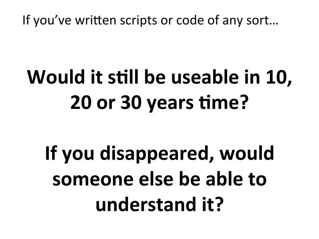
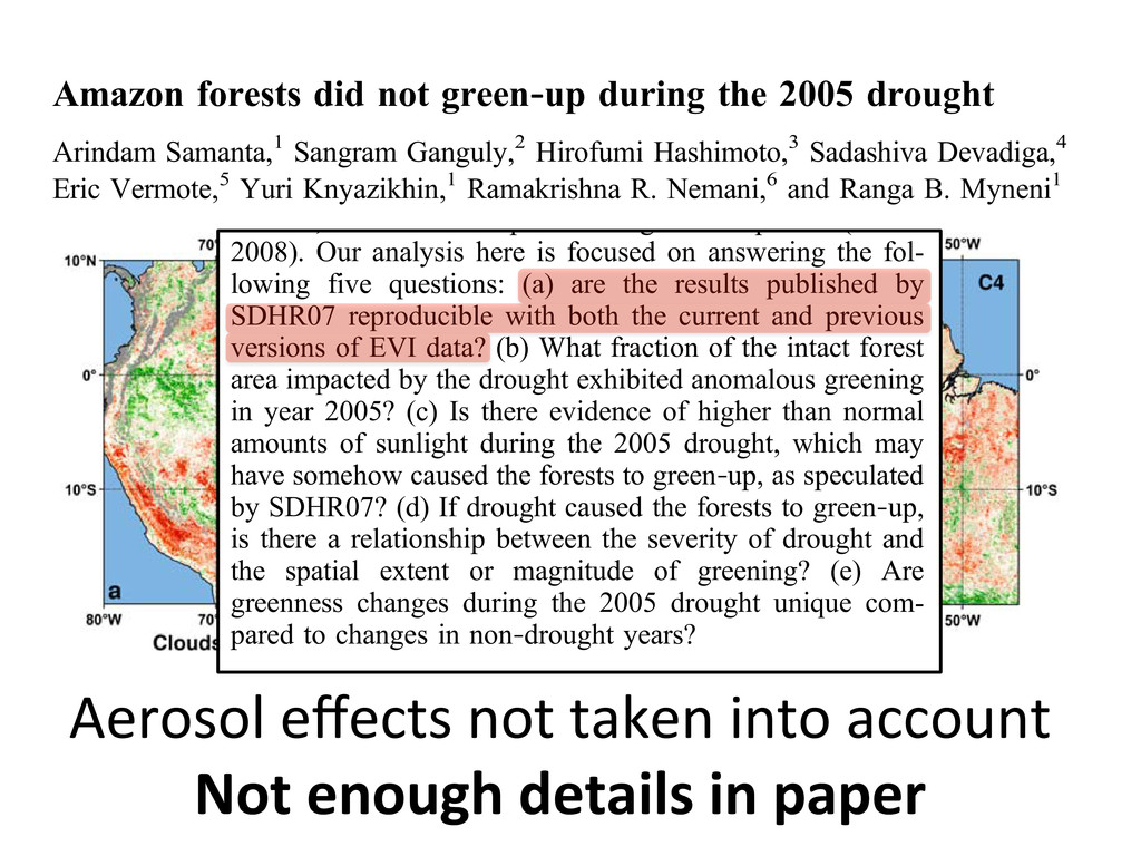
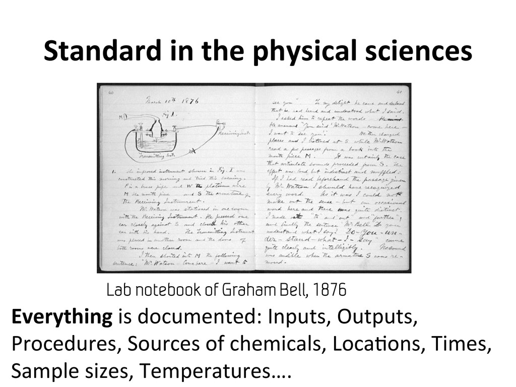
13. Aerosol optical thickness determination by exploiting the synergy of TERRA and AQUA MODIS Jiakui Tanga, Yong Xuea,b,*, Tong Yuc, Yanning Guana aLARSIS, Institute of Remote Sensing Applications, Chinese Academy of Sciences, Beijing, 100101, China bDepartment of Computing, London Metropolitan University, 166-220 Holloway Road, London N7 8DB, UK cBeijing Environmental Monitor Center, Beijing, PR China Received 23 March 2004; received in revised form 22 September 2004; accepted 25 September 2004 bstract Aerosol retrieval over land remains a difficult task because the solar light reflected by the Earth–atmospheric system mainly comes fro e ground surface. The dark dense vegetation (DDV) algorithm for MODIS data has shown excellent competence at retrieving the aeros stribution and properties. However, this algorithm is restricted to lower surface reflectance, such as water bodies and dense vegetation. s paper, we attempt to derive aerosol optical thickness (AOT) by exploiting the synergy of TERRA and AQUA MODIS data (SYNTAM hich can be used for various ground surfaces, including for high-reflective surface. Preliminary validation results by comparing wi erosol Robotic Network (AERONET) data show good accuracy and promising potential. 2004 Elsevier Inc. All rights reserved. ywords: Aerosol retrieval; Aerosol optical thickness; MODIS; TERRA; AQUA Introduction Global aerosol characterization by satellite remote sens- g arouses increasing interest, which is due to the mounting Very High Radiometer/National Oceanic and Atmospher Administration (AVHRR/NOAA; Higurashi & Nakajim 1999; Holben et al., 1992), due to new and mor sensitive instruments available like the Ocean Color an the AOT of the northeast of Beijing is greater than of the others, which demonstrates the larger temporal variability of the aerosol. Fig. 3. The flowchart of aerosol retrieval by SYNTAM. J. Tang et al. / Remote Sensing of Environment 94 (2005) 327–334 331 nd Haigh (1995) proposed that the surface approximated by a part that describes the h the wavelength and a part that describes with the geometry. Under this assumption, wo views’ surface reflectance can be written 2;ki ð7Þ s the surface reflectance for the first view the second view. The ratio K is assumed to on the variation of the surface reflectance metry and to be independent of the wave- rdew & Haigh, 1995; Veefkind et al., 1998, se aerosol extinction decreases rapidly with he AOT at 2.13 Am will be very small as the AOT in the visible. This assumption alid when the aerosol is dominated by the such as desert dust. Ignoring the atmos- ibution at 2.13 Am, Kk=2.13 Am can ated as the ratio between the top of the eflectances for the two overpasses at this Since K is assumed independent of the his value for Kk=2.13 Am can also be used le channels (0.47, 0.55, 0.66 Am), which k=2.13 Am . Actually, it is very difficult to directly get the analytical solution of nonlinear Eq. (6). However, an approximate numerical solution can be obtained by means of many numerical methods. In this paper, Newton iteration algo- rithm is used for our solution. 3. Data and processing MODIS is one of the sensors on board EOS-AM1/ TERRA and EOS-PM1/AQUA, which are both sun- synchronous polar orbiting satellites. TERRA was launched on Dec. 12, 1999 and flies northward pass the equator at about local time 10:30 AM. AQUA, launched Fig. 2. Aqua/MODIS reflectance RGB (R for Band 1; G for Band 4; B for Band 3) composed image (400æ400), Gaussian enhancement is made. er equations consists in substituting the exact ial equation for radiant intensity by common ations for the upward and incident radiation neral solution of this problem has been given (1969). Therefore, we can find the relation round surface reflectance A and apparent lectance on the top of atmosphere) AV, which Xue and Cracknell (1995) as follows: þ a 1 À AV ð Þe aÀb ð Þesk 0 sechV þ b 1 À AV ð Þe aÀb ð Þesk 0 sechV ð2Þ and b=2, e is the backscattering coefficient, The solar zenith angle is calculated from ude, and satellite pass time or the data set for tration of aerosol particles, namely, Angstrom’s tur- bidity coefficient b. Now, if we substitute bitemporal satellite data such as three visible spectral bands data, central wavelength of 0.47, 0.55, 0.66 Am, respectively, from TERRA and AQUA into Eq. (2), we can obtain one group of nonlinear equations as follows: Aj;ki ¼ Aj;ki Vb À aj À Á þ aj 1 À Aj;ki V À Áe aj Àb ð Þe 0:00879kÀ4:09 i þb j kÀa i ð Þsechj V Aj;ki Vb À aj À Á þ b 1 À Aj;ki V À Áe aj Àb ð Þe 0:00879kÀ4:09 i þb j kÀa i ð Þsechj V ð6Þ where j=1,2, respectively, stand for the observation of TERRA-MODIS and AQUA-MODIS; i=1,2,3, respectively, other symbols are defined in the Appendix A. In real conditions, the bidirectional reflectance proper- ties of the ground surface depend not only on the wavelength but also on the geometry. For two successive views of TERRA and AQUA, the geometries often are different, hence we have to take account of this influence. Flowerdew and Haigh (1995) proposed that the surface reflectance be approximated by a part that describes the variation with the wavelength and a part that describes the variation with the geometry. Under this assumption, the ratio of two views’ surface reflectance can be written as follows: Kki ¼ A1;ki =A2;ki ð7Þ where A1,k i is the surface reflectance for the first view and A2,k i for the second view. The ratio K is assumed to depend only on the variation of the surface reflectance with the geometry and to be independent of the wave- length (Flowerdew & Haigh, 1995; Veefkind et al., 1998, 2000). Because aerosol extinction decreases rapidly with wavelength, the AOT at 2.13 Am will be very small as compared to the AOT in the visible. This assumption will not be valid when the aerosol is dominated by the coarse mode, such as desert dust. Ignoring the atmos- pheric contribution at 2.13 Am, Kk=2.13 Am can be approximated as the ratio between the top of the atmosphere reflectances for the two overpasses at this wavelength. Since K is assumed independent of the wavelength, this value for Kk=2.13 Am can also be used Not  enough   informa:on  to   reproduce!  
14. Standard  in  the  physical  sciences   ed in ce the rk-flow: t Lab notebook of Graham Bell, 1876 Everything  is  documented:  Inputs,  Outputs,   Procedures,  Sources  of  chemicals,  Loca@ons,  Times,   Sample  sizes,  Temperatures….  
15. What  about  remote  sensing?   “An unsupervised classification was performed…”!   What  algorithm?   How  many  classes?   How  many  itera@ons?   What  termina@on  parameters?  
16. How  to  make  research  reproducible?   1.  Do  it  in  code   – If  everything  from  data  import  through  processing   to  crea@ng  a  graph/table  is  done  in  code  then  it   can  be  ‘one-­‐click’  reproducible     2.  Document  it   – Very  thoroughly!  Every  single  parameter,  every   opera@on.  Every  piece  of  data  used  as  input.   – (Electronically,  on  paper  –  whatever)  
17. Then  share  it  with  people…     •  Supplementary  Informa@on  with  a  journal   paper  -­‐>  Soon  to  be  a  requirement?   •  In  an  Appendix  to  a  paper/thesis   •  On  your  personal  webpage     Doesn’t  really  maNer  where  it  is  as  long  as:   •  People  can  get  hold  of  it   •  People  know  where  to  look  
18. Example:  GPS  Precipitable  Water   •  Valida@on  of  a  new  &  novel  data  source   against  AERONET  &  Radiosonde  data   •  Method  must  be  robust,  accurate,  repeatable   etc.   Bri:sh  Isles   GNSS  Facility  
19. R  Code:   library(ProjectTemplate) load.project() All  graphs   All  tables   All  automa:cally  produced   ‘One  Click’  Reproducibility   (+  comments/docs)  
20. Example:  ArcGIS  provenance  tool   “I’ve forgotten what I did to create Output3.tif”! “I can’t remember the parameters I used for the unsupervised classification”! Data  Provenance  
21. What  happened,  when,  how     1434:  pain@ng  dated  by  van  Eyck;   1516:  in  possession  of  Don  Diego  de   Guevara,  a  Spanish  career  cour@er  of  the   Habsburgs;   1516:  portrait  given  to  Margaret  of  Austria,   Habsburg  Regent  of  the  Netherlands;   1530:  inherited  by  Margaret’s  niece  Mary   of  Hungary;   1558:  inherited  by  Philip  II  of  Spain;   1599:  on  display  in  the  Alcazar  Palace  in   Madrid;   1794:  now  in  the  Palacio  Nuevo  in  Madrid;   1816:  in  London,  probably  plundered  by  a   certain  Colonel  James  Hay  a=er  the  BaNle  of   Vitoria  (1813),  from  a  coach  loaded  with  easily   portable  artworks  by  King  Joseph  Bonaparte;   1841:  the  pain@ng  was  included  in  a  public   exhibi@on;   1842:  bought  by  the  Na@onal  Gallery,   London  for  £600,  where  it  remains.  
23. Field  spectra  collected  in  1989  used  in  my  PhD  
24. Sustainability   Data   Code   Methods  
25. Formats   Metadata   Sustainable   Data  
26. Metadata  –  What  is  this  crazy  data?   Source   Units   Loca@on   Date/ Time   Person   Method   General  Notes  &  Explana@on  
27. How  to  store  metadata   •  Inside  the  file   – Almost  all  formats  can  store  georeferencing   – ENVI  header  files  can  store  Sensor,  Wavelengths,   FWHMs,  Units  and  more…   – ArcGIS  geodatabases  can  store  metadata   •  In  a  metadata  database   – Name  of  file  -­‐>  List  of  metadata     README  files:  Simple  +  Effec@ve  
28. How  to  choose  a  format?   ASCII   Simple  Text   No  special  chars   Binary  +   Header   ENVI  files   Well-­‐known  format   TIFF   SHP  
29. Beware  of  ‘Well-­‐known  formats’   The  most   popular  word   processor  in  the   1980s…   …Can  you  read   its  files  now?     OPEN  formats   are  beler  
30. How  to  code  sustainably?   Good  Design,  Commen@ng,  Version  Control,   Automated  Tes@ng…         Best  Prac:ces  for  Scien:fic  Compu:ng:   hNp://arxiv.org/pdf/1210.0530.pdf   Do you spend too much time wrestling with computers, and not enough doing research? We can help
31. So  what?   This  stuff  is  important  for  you  and  for  others   Think  about  it!   (tell  others  about  it)     Read  up  about  it   (www.rtwilson.com/academic/rr)    
32. Easy  Idea:   Spend  an  a-ernoon  crea:ng  some  README   files  in  your  work  folders:   •  What  is  this?   •  Where  did  it  come  from?   •  What  did  I  do  with  it?   •  What  do  I  need  to   remember  in  a  year   about  it?  
33. Easy  Idea:   Hide  your  results/outputs  and  try  and   reproduce  them  again  –  check  they’re   exactly  the  same   •  What  did  you  need  to  know  that  wasn’t   wriNen  down?   •  Write  that  down   somewhere  before   you  forget!  
34. Harder  Idea:   Script/Automate  some  of  your  work  –  then   it’s  easier  to  repeat,  and  self-­‐documen:ng   •  Use  the  ArcGIS  Model  Builder  (can  use   ENVI  commands  too!)   •  Learn  some  basic   coding  (eg.  Python)   •  If  that  isn’t  possible   then  document  it   thoroughly  
35. Harder  Idea:   Look  at  the  So-ware  Carpentry  lessons  –  can   you  apply  those  to  your  code?   •  Does  it  have  comments?   •  Do  you  know  what  the  dependencies  are?   •  Does  it  have  tests?   •  Is  it  under  version   control?  
36. Prac:cal  Ideas:   •  Spend  an  a=ernoon  crea@ng  some  README  files   in  your  work  folders   •  Hide  your  results/outputs  and  try  and  reproduce   them  again  –  check  they’re  exactly  the  same   •  Script/Automate  some  of  your  work  –  then  it’s   easier  to  repeat,  and  self-­‐documen@ng   •  Look  at  the  So=ware  Carpentry  lessons  –  can  you   apply  those  to  your  code?   robin@rtwilson.com   www.rtwilson.com/academic/rr