Neural Networks (CNN). • Learn how to apply CNN to to visual detection and recognition tasks. • Learn how to apply Transfer learning with image and language data. • Understand how to implement Convolution Neural Network using Pytorch framework. 2
a universal function approximator which can be used for classification or regression problem. • They build up complex pattern from simple pattern hierachically. • Each layer learn to detect simple combination of pattern detected by previous layer. • The lowest layers of the model capture simple patterns where the next layers capture more complex pattern. 3
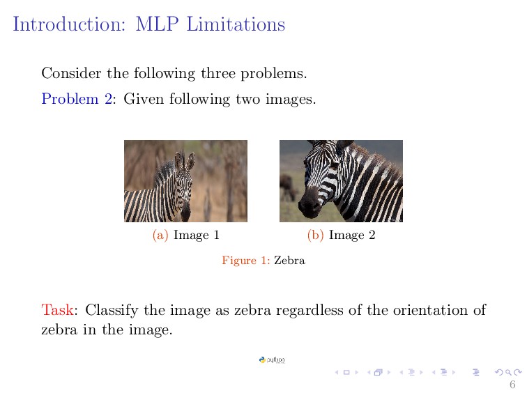
Given following two images. (a) Image 1 (b) Image 2 Figure 1: Zebra Task: Classify the image as zebra regardless of the orientation of zebra in the image. 6
is very challenging. 1 Require a very large network 2 MLPs are sensitive to the location of the pattern • Moving it by one component results in an entirely different input that the MLP wont recognize. In many problems the location of a pattern is not important • Only the presence of the pattern. • Requirement: Network must be shift invariant. More details 7
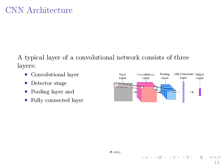
designed specifically for such problems: • Handle very high input dimension • Exploit the 2D topology of image or 3D topology for video data. • Build in invariance to certain variations we expect (translations, illumination etc) 8
networks for processing visual data. • They employs a mathematical operation called convolution in place of general matrix multiplication in at least one of their layers. • CNNs are often used for 2D or 3D data (such as grayscale or RGB images), but can also be applied to several other types of input, such as: 1 1D data: time-series, raw waveforms 2 2D data: grayscale images, spectrograms 3 3D data: RGB images, multichannel spectrograms 9
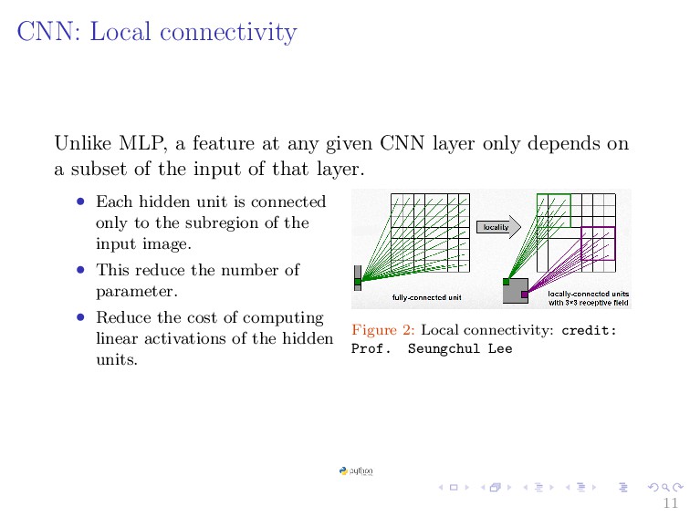
CNN layer only depends on a subset of the input of that layer. • Each hidden unit is connected only to the subregion of the input image. • This reduce the number of parameter. • Reduce the cost of computing linear activations of the hidden units. Figure 2: Local connectivity: credit: Prof. Seungchul Lee 11
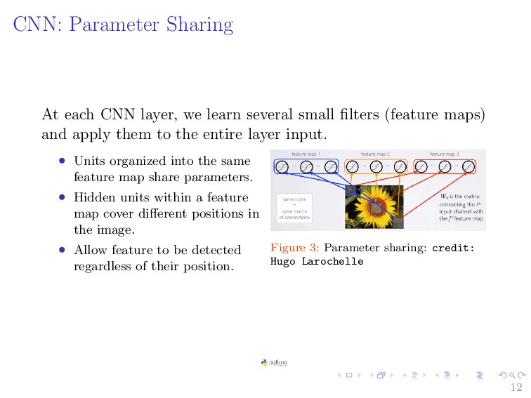
small filters (feature maps) and apply them to the entire layer input. • Units organized into the same feature map share parameters. • Hidden units within a feature map cover different positions in the image. • Allow feature to be detected regardless of their position. Figure 3: Parameter sharing: credit: Hugo Larochelle 12
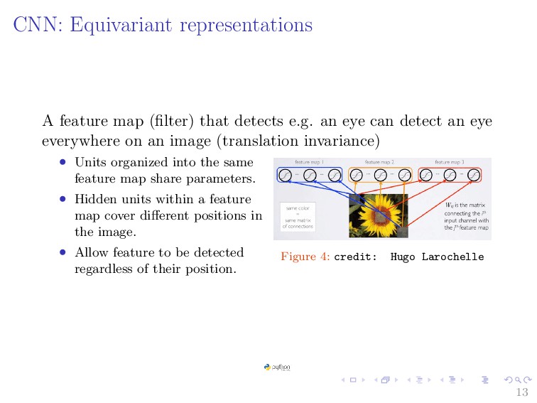
an eye can detect an eye everywhere on an image (translation invariance) • Units organized into the same feature map share parameters. • Hidden units within a feature map cover different positions in the image. • Allow feature to be detected regardless of their position. Figure 4: credit: Hugo Larochelle 13
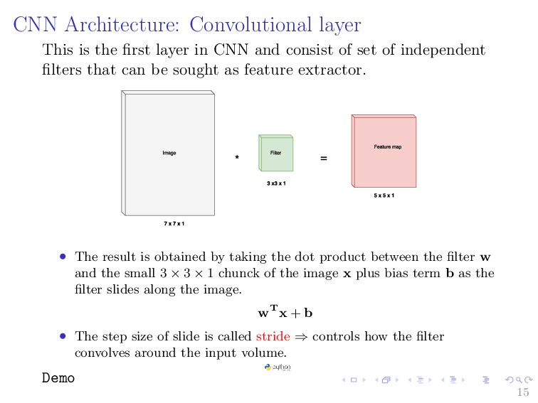
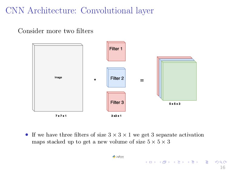
CNN and consist of set of independent filters that can be sought as feature extractor. • The result is obtained by taking the dot product between the filter w and the small 3 × 3 × 1 chunck of the image x plus bias term b as the filter slides along the image. wTx + b • The step size of slide is called stride ⇒ controls how the filter convolves around the input volume. Demo 15
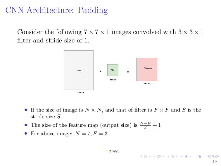
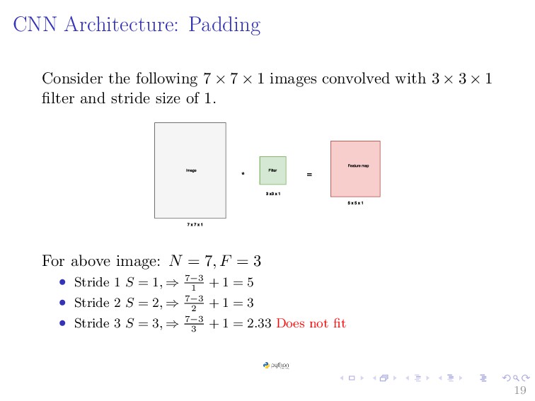
1 images convolved with 3 × 3 × 1 filter and stride size of 1. • If the size of image is N × N, and that of filter is F × F and S is the stride size S. • The size of the feature map (output size) is N−F S + 1 • For above image: N = 7, F = 3 18
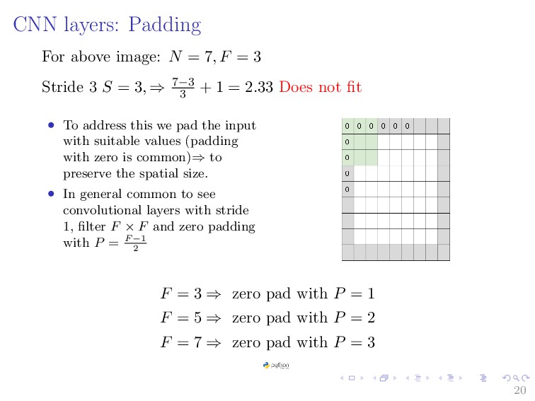
= 3 Stride 3 S = 3, ⇒ 7−3 3 + 1 = 2.33 Does not fit • To address this we pad the input with suitable values (padding with zero is common)⇒ to preserve the spatial size. • In general common to see convolutional layers with stride 1, filter F × F and zero padding with P = F −1 2 F = 3 ⇒ zero pad with P = 1 F = 5 ⇒ zero pad with P = 2 F = 7 ⇒ zero pad with P = 3 20
a volume of size W1 × H1 × D1 • Requires four hype-parameters: 1 Number of filters K. 2 Spatial extent of filter F. 3 Amount zero padding P. Common settings: • K = (power of 2 e.g) 4, 8, 16, 32, 64, 128 • F = 3, S = 1, P = 1 • F = 5, S = 1, P = 2 • F = 5, S = 2, P =? whatever fits. • Produce a volume of size W2 × H2 × D2 where W2 = (W1 − F + 2P)/S + 1 H2 = (H1 − F + 2P)/S + 1 D2 = K • The number of weights per filter is F · F · D1 and the total number of parameters is (F · F · D1 ) · K and K biases. 21
a volume of size W1 × H1 × D1 • Requires four hype-parameters: 1 Number of filters K. 2 Spatial extent of filter F. 3 Amount zero padding P. Common settings: • K = (power of 2 e.g) 4, 8, 16, 32, 64, 128 • F = 3, S = 1, P = 1 • F = 5, S = 1, P = 2 • F = 5, S = 2, P =? whatever fits. • Produce a volume of size W2 × H2 × D2 where W2 = (W1 − F + 2P)/S + 1 H2 = (H1 − F + 2P)/S + 1 D2 = K • The number of weights per filter is F · F · D1 and the total number of parameters is (F · F · D1 ) · K and K biases. 21
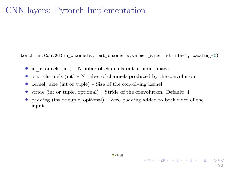
(int) – Number of channels in the input image • out_channels (int) – Number of channels produced by the convolution • kernel_size (int or tuple) – Size of the convolving kernel • stride (int or tuple, optional) – Stride of the convolution. Default: 1 • padding (int or tuple, optional) – Zero-padding added to both sides of the input. 22
of a conv layer is run through a non-linear function. • ReLU function is often used after every convolution operation. • It replace all the negative pixel in the feature map by zero. 23
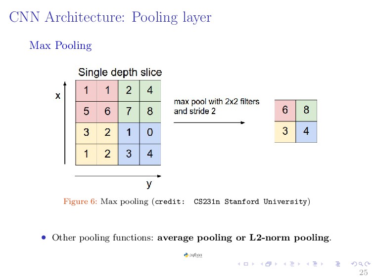
filter ⇒ takes each feature map from a convolution layer produce a condensed feature map. • Make representation smaller and more manageable. • Operates over each activation map independently • Reduce computational cost and the amount of parameter. • Preserve spatial invariance. 24
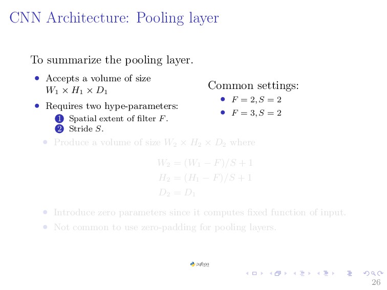
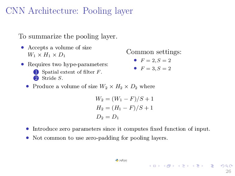
Accepts a volume of size W1 × H1 × D1 • Requires two hype-parameters: 1 Spatial extent of filter F. 2 Stride S. Common settings: • F = 2, S = 2 • F = 3, S = 2 • Produce a volume of size W2 × H2 × D2 where W2 = (W1 − F)/S + 1 H2 = (H1 − F)/S + 1 D2 = D1 • Introduce zero parameters since it computes fixed function of input. • Not common to use zero-padding for pooling layers. 26
Accepts a volume of size W1 × H1 × D1 • Requires two hype-parameters: 1 Spatial extent of filter F. 2 Stride S. Common settings: • F = 2, S = 2 • F = 3, S = 2 • Produce a volume of size W2 × H2 × D2 where W2 = (W1 − F)/S + 1 H2 = (H1 − F)/S + 1 D2 = D1 • Introduce zero parameters since it computes fixed function of input. • Not common to use zero-padding for pooling layers. 26
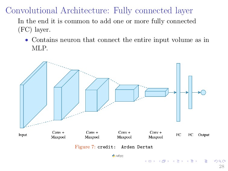
common to add one or more fully connected (FC) layer. • Contains neuron that connect the entire input volume as in MLP. Figure 7: credit: Arden Dertat 28
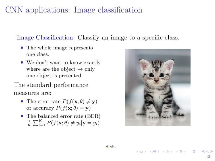
a specific class. • The whole image represents one class. • We don’t want to know exactly where are the object → only one object is presented. The standard performance measures are: • The error rate P(f(x; θ) = y) or accuracy P(f(x; θ) = y) • The balanced error rate (BER) 1 K K i=1 P(f(x; θ) = yi |y = yi ) 30
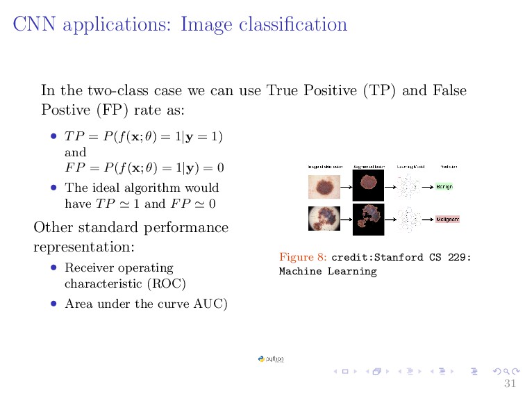
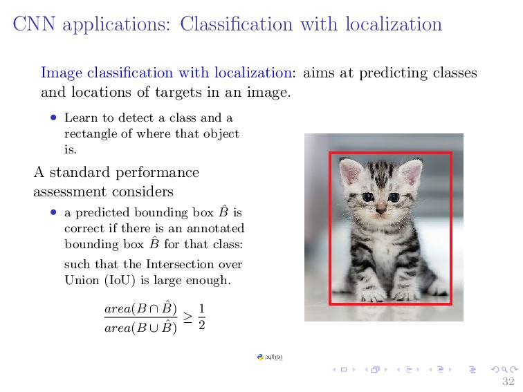
at predicting classes and locations of targets in an image. • Learn to detect a class and a rectangle of where that object is. A standard performance assessment considers • a predicted bounding box ˆ B is correct if there is an annotated bounding box ˆ B for that class: such that the Intersection over Union (IoU) is large enough. area(B ∩ ˆ B) area(B ∪ ˆ B) ≥ 1 2 32
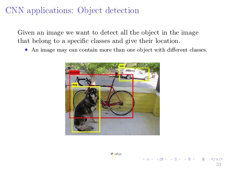
detect all the object in the image that belong to a specific classes and give their location. • An image may can contain more than one object with different classes. 33
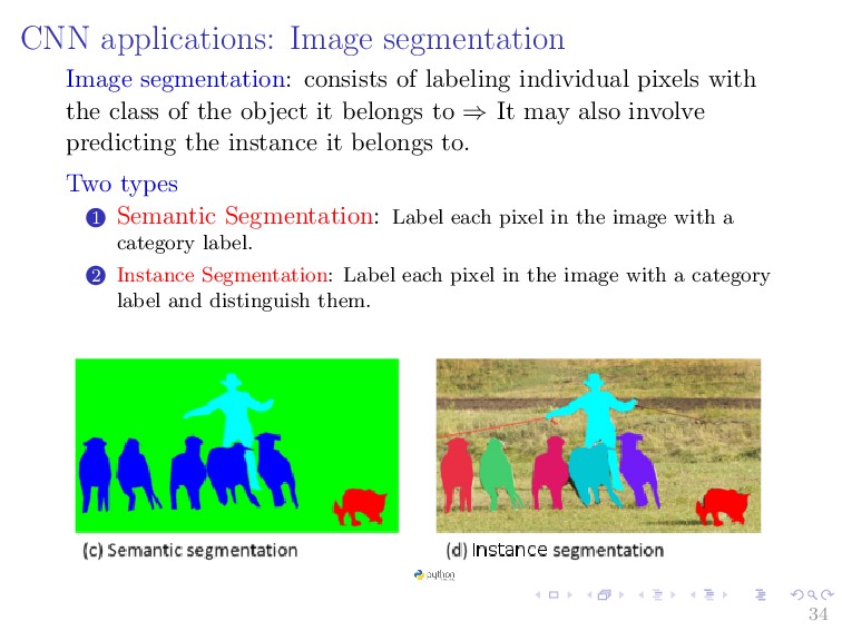
pixels with the class of the object it belongs to ⇒ It may also involve predicting the instance it belongs to. Two types 1 Semantic Segmentation: Label each pixel in the image with a category label. 2 Instance Segmentation: Label each pixel in the image with a category label and distinguish them. 34
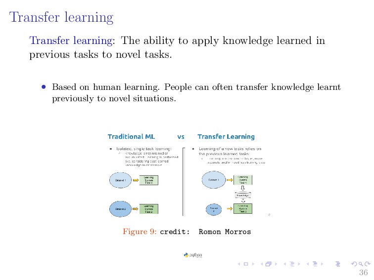
in previous tasks to novel tasks. • Based on human learning. People can often transfer knowledge learnt previously to novel situations. Figure 9: credit: Romon Morros 36
network from scratch for your task: • Take a network trained on a different domain for a different source task. • Adapt it for your domain and your target task. • A popular approach in computer vision and natural language processing task. 37
an entire CNN from scratch (with random initialization) ⇒ (computation time and data availability) • Very Deep Networks are expensive to train.For example, training ResNet18 for 30 epochs in 4 NVIDIA K80 GPU took us 3 days. • Determining the topology/flavour/training method/hyper parameters for deep learning is a black art with not much theory to guide you. 38
TelecomBCN Bercelona(winter 2017) • 6.S191 Introduction to Deep Learning: MIT 2018. • Deep learning Specilization by Andrew Ng: Coursera • Introductucion to Deep learning: CMU 2018 • Cs231n: Convolution Neural Network for Visual Recognition: Stanford 2018 • Deep learning in Pytorch, Francois Fleurent: EPFL 2018 39