set out by the Clay Mathematics Institute • The Millenium Prize Problems are now six unsolved problems and one solved problem. • They have a certain level of infamy due to the Clay Mathematics Institute’s promise of $1 million for a correct proof of any of the problems 2
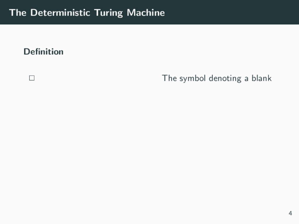
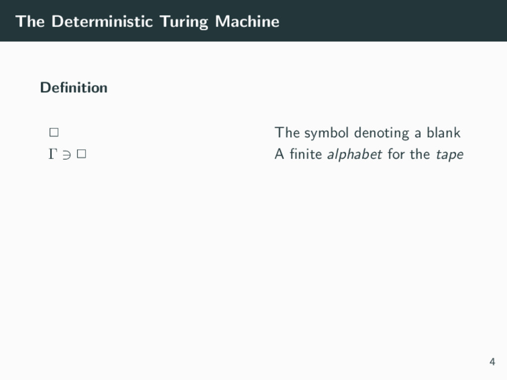
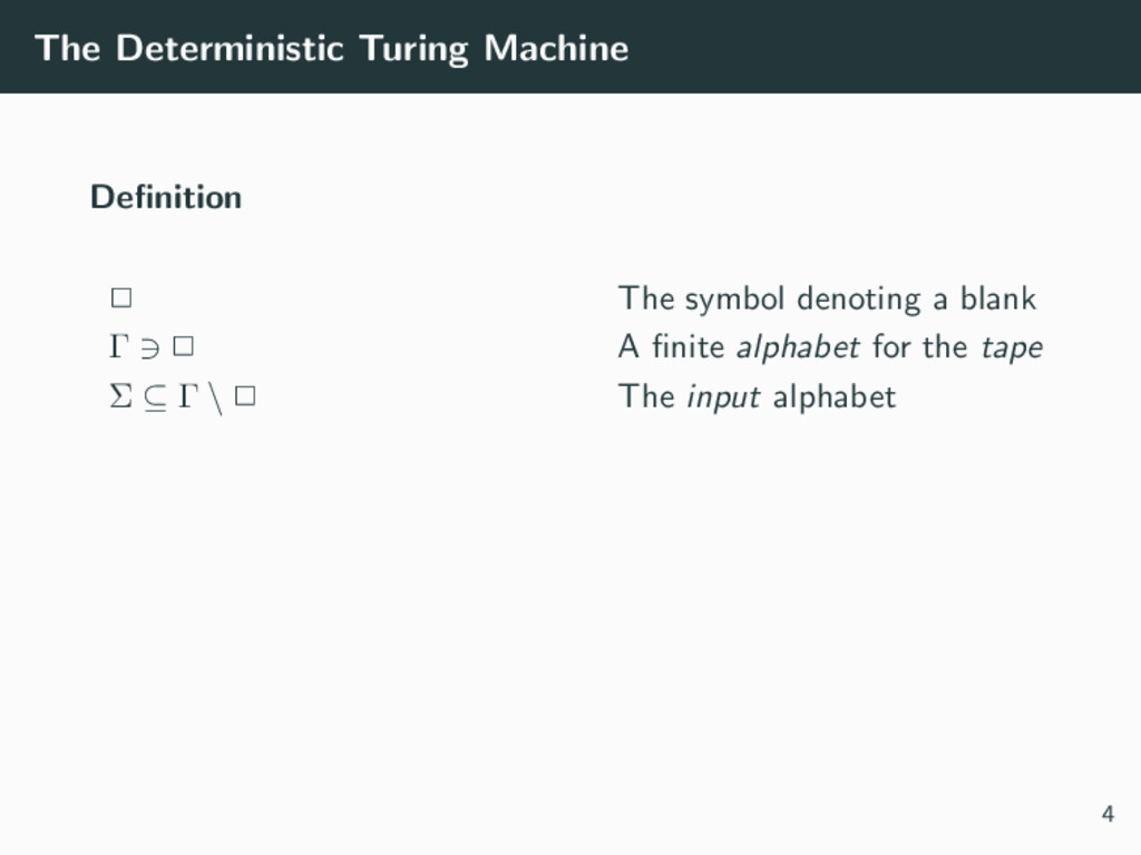
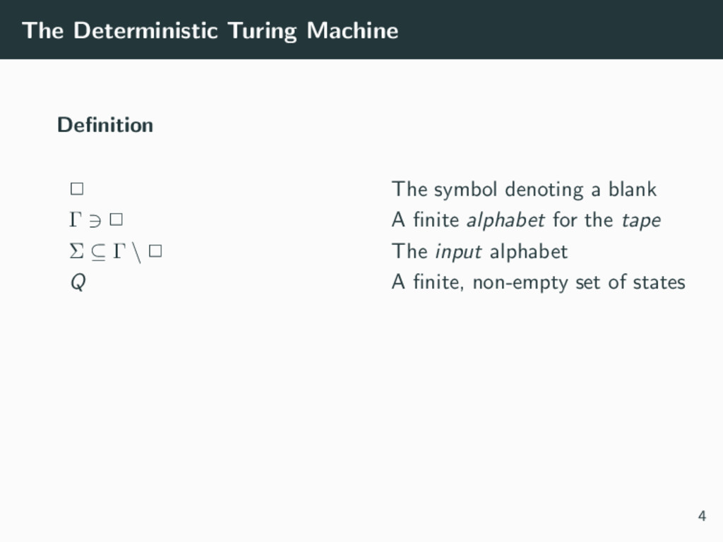
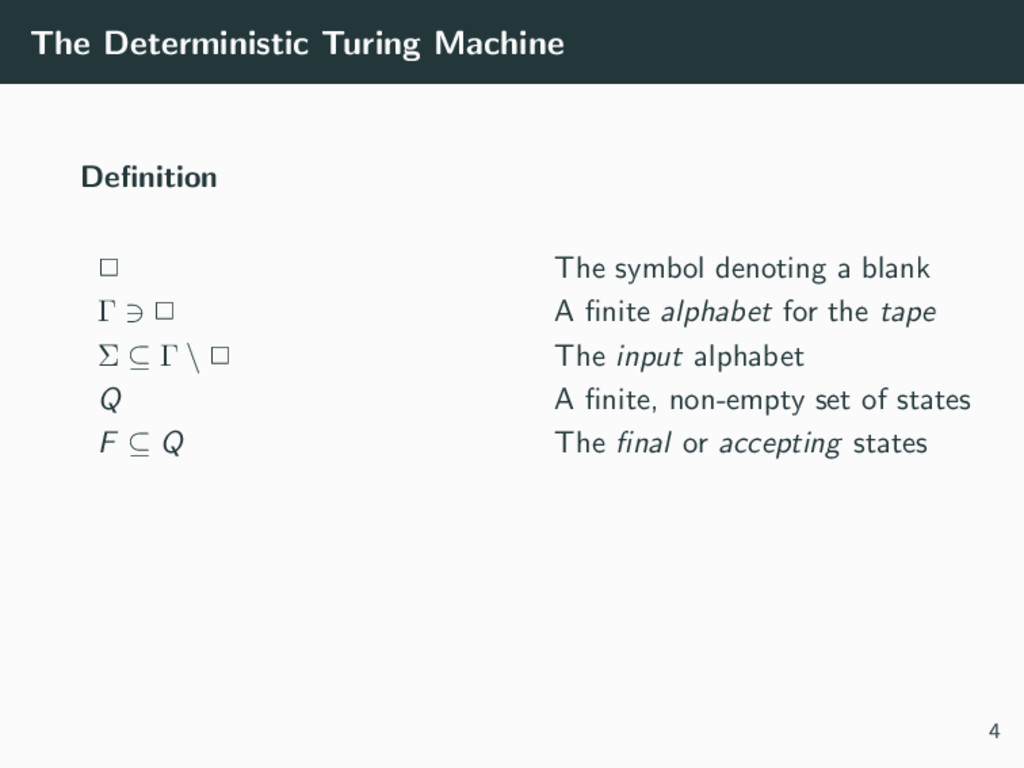
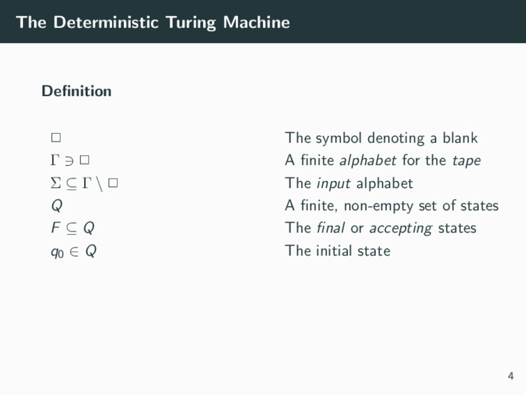
blank Γ 2 A finite alphabet for the tape Σ ⊆ Γ \ 2 The input alphabet Q A finite, non-empty set of states F ⊆ Q The final or accepting states q0 ∈ Q The initial state 4
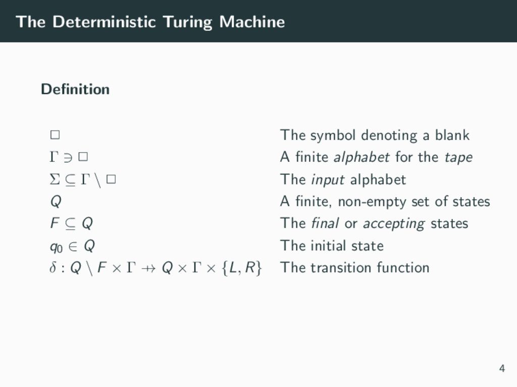
blank Γ 2 A finite alphabet for the tape Σ ⊆ Γ \ 2 The input alphabet Q A finite, non-empty set of states F ⊆ Q The final or accepting states q0 ∈ Q The initial state δ : Q \ F × Γ → Q × Γ × {L, R} The transition function 4
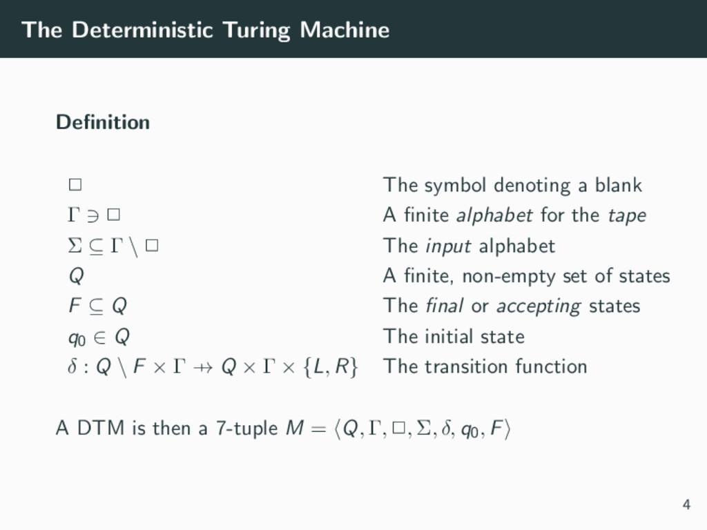
blank Γ 2 A finite alphabet for the tape Σ ⊆ Γ \ 2 The input alphabet Q A finite, non-empty set of states F ⊆ Q The final or accepting states q0 ∈ Q The initial state δ : Q \ F × Γ → Q × Γ × {L, R} The transition function A DTM is then a 7-tuple M = Q, Γ, 2, Σ, δ, q0, F 4
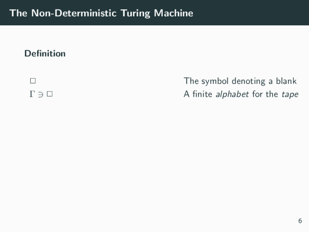
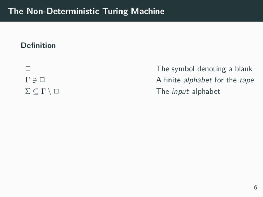
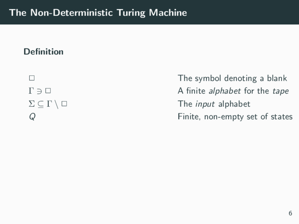
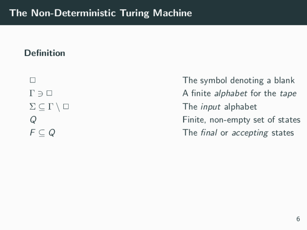
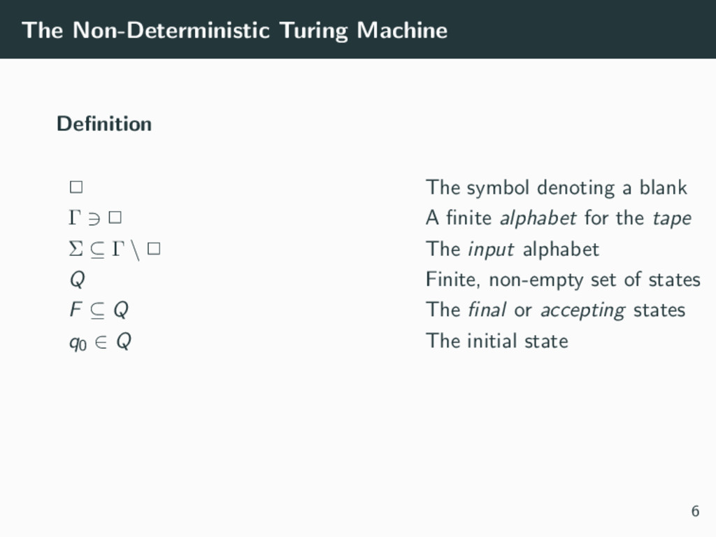
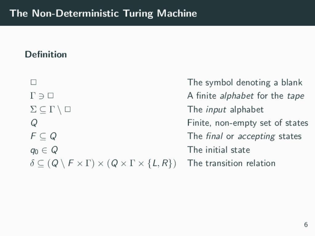
blank Γ 2 A finite alphabet for the tape Σ ⊆ Γ \ 2 The input alphabet Q Finite, non-empty set of states F ⊆ Q The final or accepting states q0 ∈ Q The initial state 6
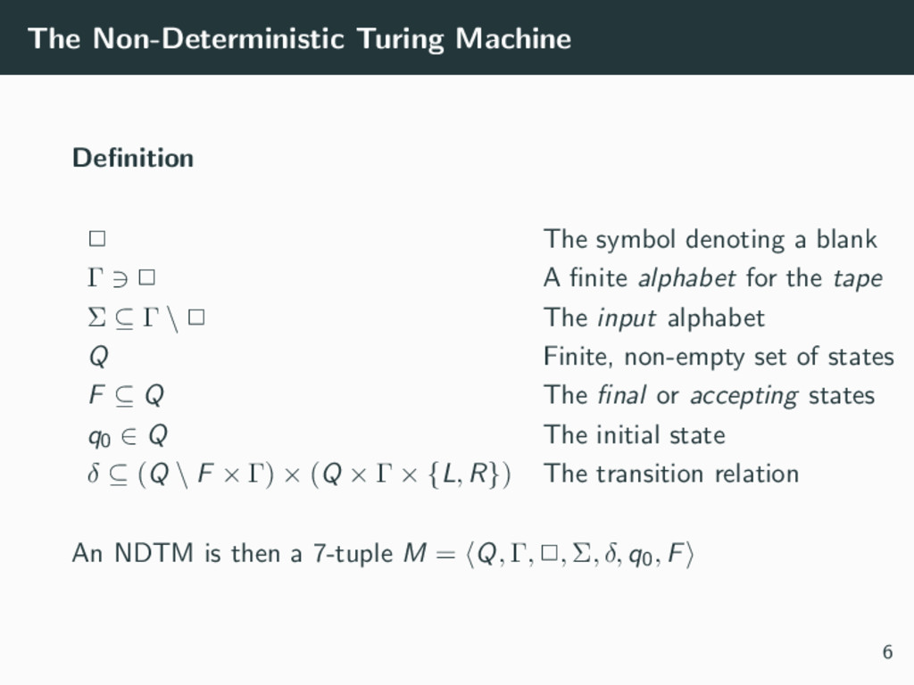
blank Γ 2 A finite alphabet for the tape Σ ⊆ Γ \ 2 The input alphabet Q Finite, non-empty set of states F ⊆ Q The final or accepting states q0 ∈ Q The initial state δ ⊆ (Q \ F × Γ) × (Q × Γ × {L, R}) The transition relation 6
blank Γ 2 A finite alphabet for the tape Σ ⊆ Γ \ 2 The input alphabet Q Finite, non-empty set of states F ⊆ Q The final or accepting states q0 ∈ Q The initial state δ ⊆ (Q \ F × Γ) × (Q × Γ × {L, R}) The transition relation An NDTM is then a 7-tuple M = Q, Γ, 2, Σ, δ, q0, F 6
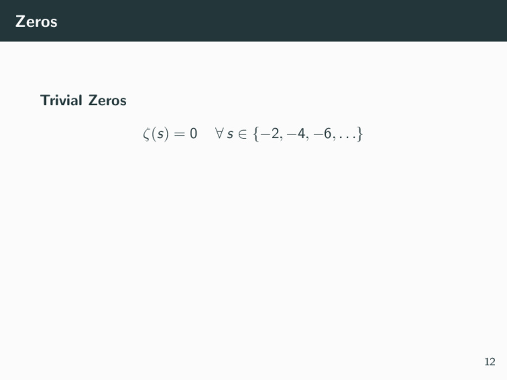
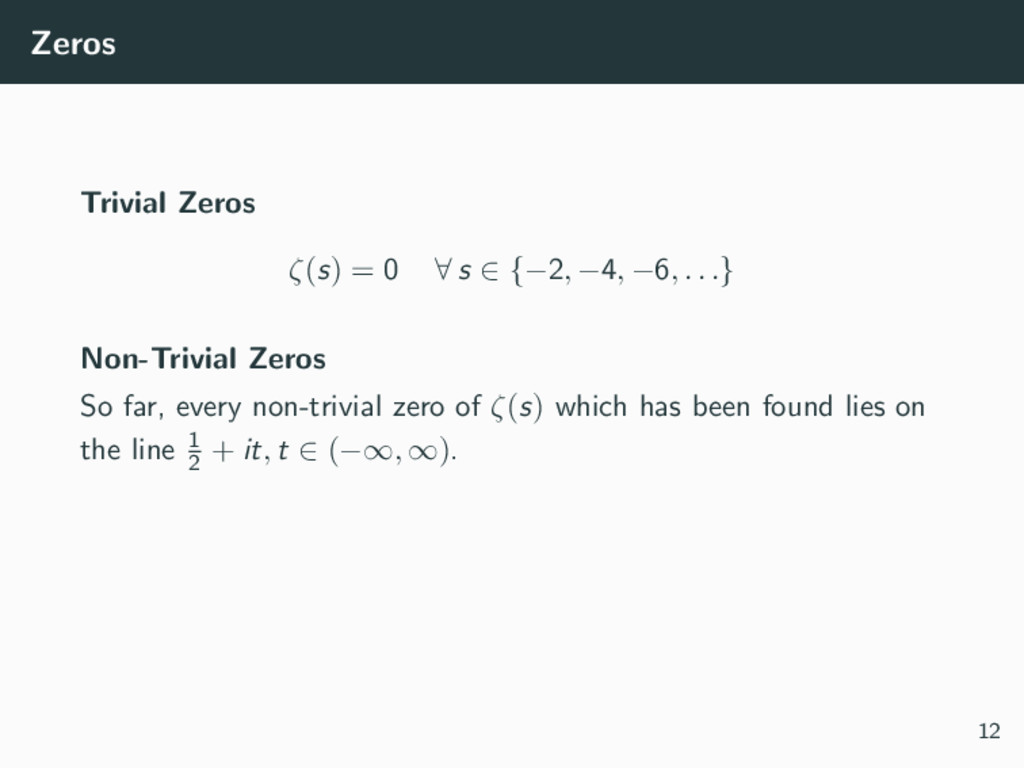
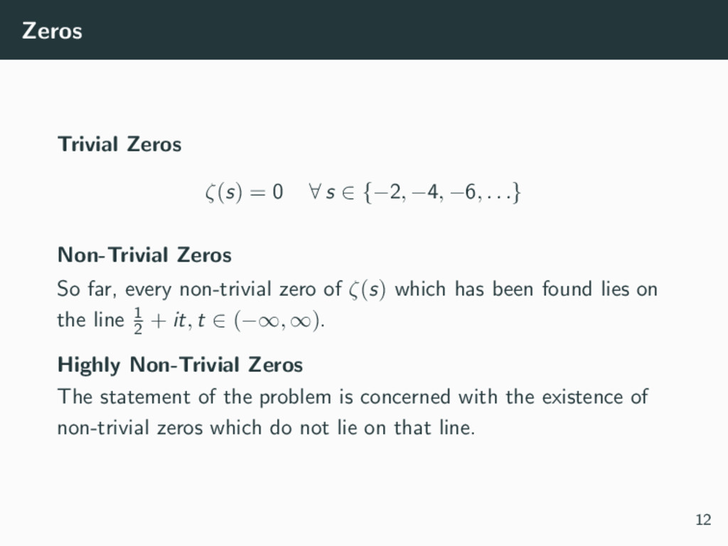
−4, −6, . . .} Non-Trivial Zeros So far, every non-trivial zero of ζ(s) which has been found lies on the line 1 2 + it, t ∈ (−∞, ∞). Highly Non-Trivial Zeros The statement of the problem is concerned with the existence of non-trivial zeros which do not lie on that line. 12
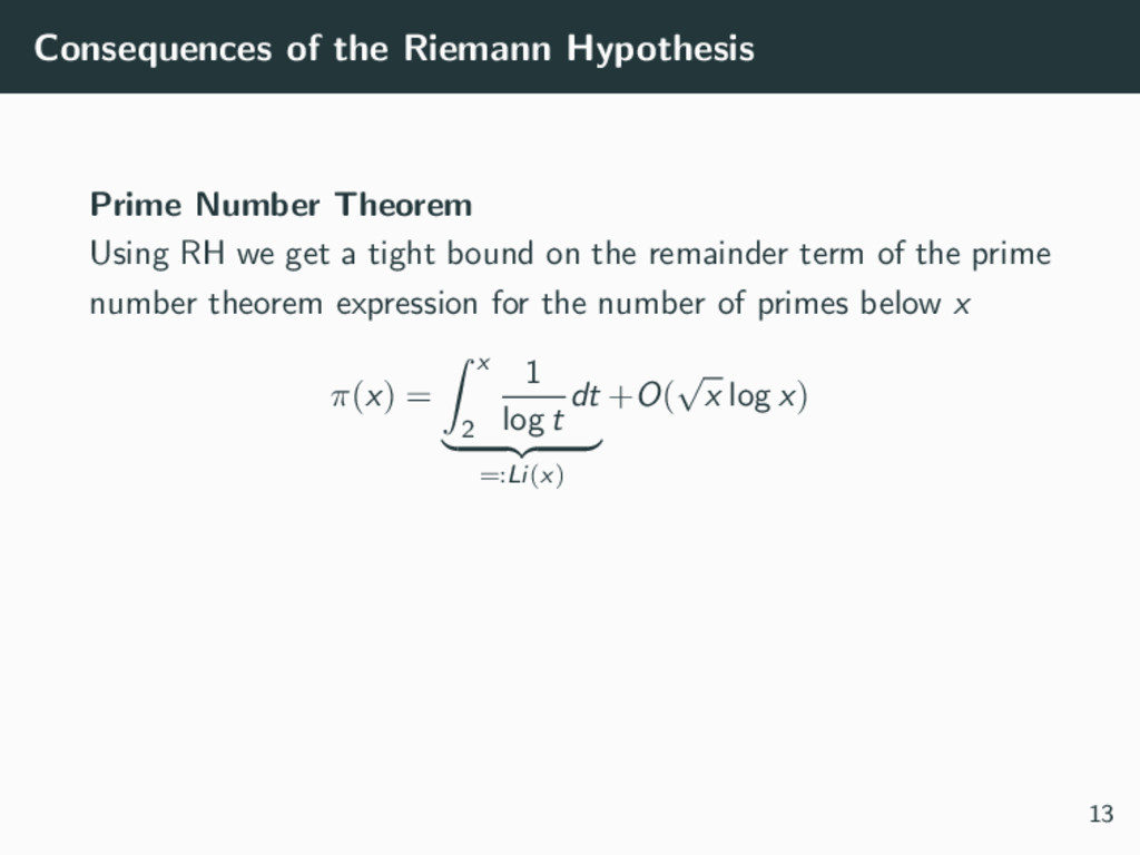
we get a tight bound on the remainder term of the prime number theorem expression for the number of primes below x π(x) = x 2 1 log t dt =:Li(x) +O( √ x log x) 13
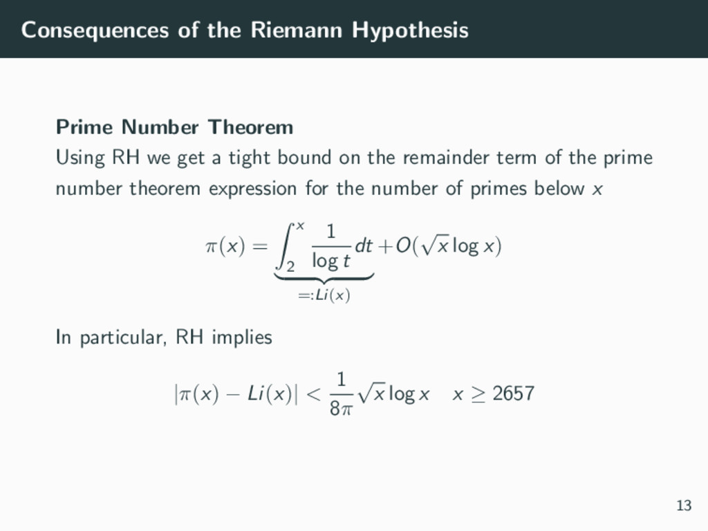
we get a tight bound on the remainder term of the prime number theorem expression for the number of primes below x π(x) = x 2 1 log t dt =:Li(x) +O( √ x log x) In particular, RH implies |π(x) − Li(x)| < 1 8π √ x log x x ≥ 2657 13
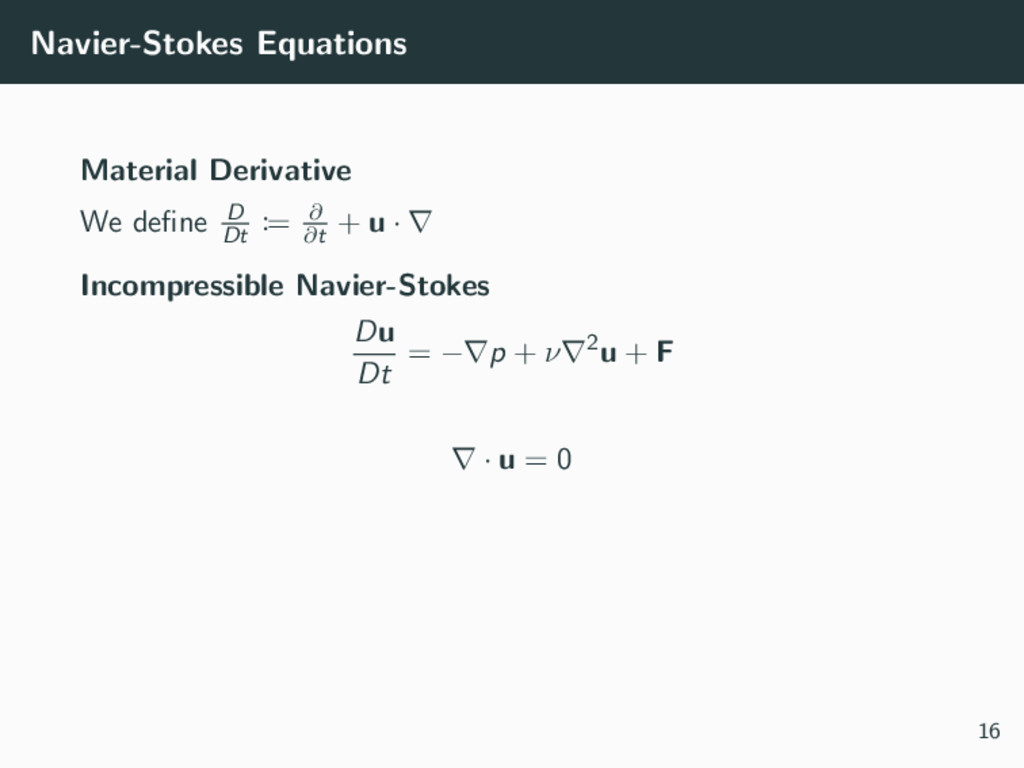
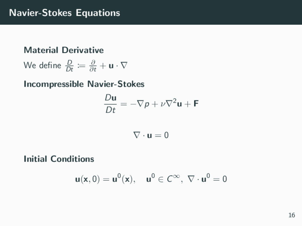
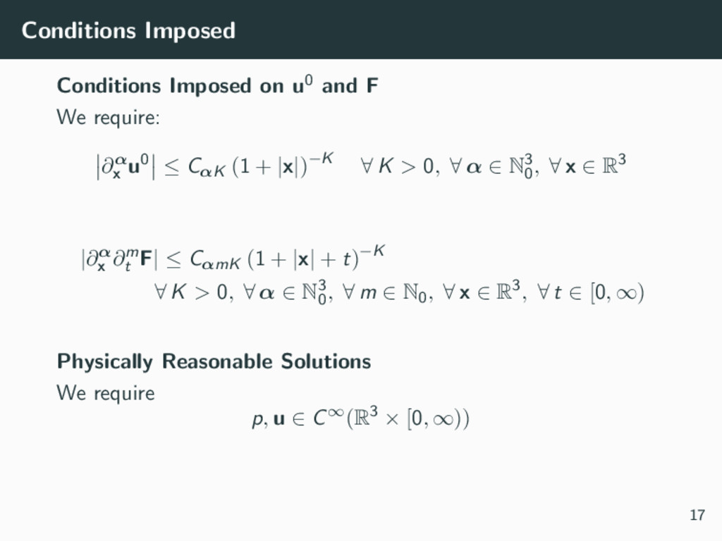
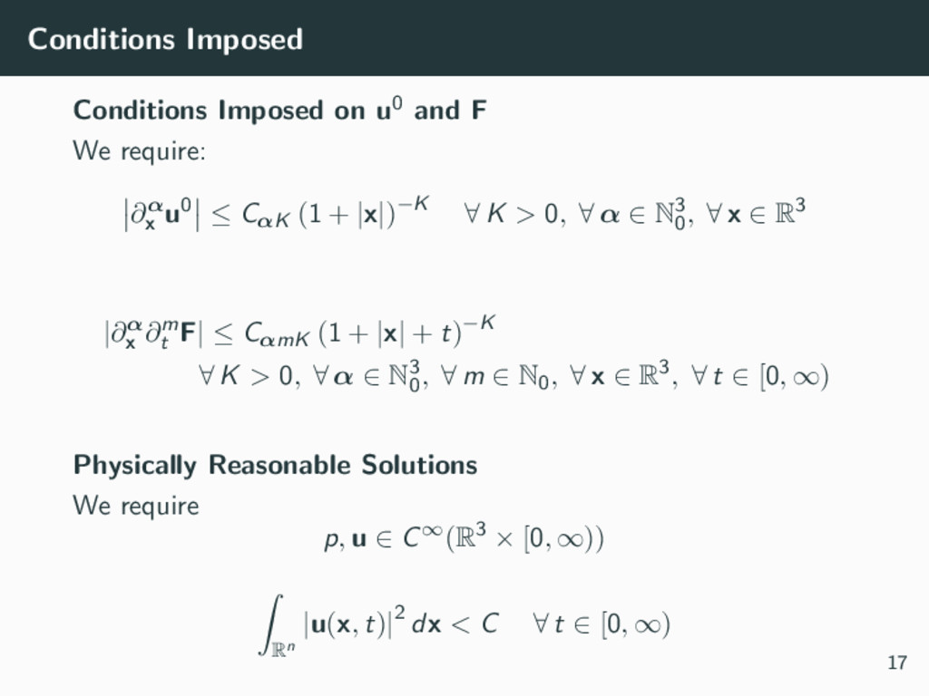
smooth solutions with finite energy of the Navier-Stokes equations for any given divergence-free initial velocity field with no external force applied on either R3 or R3/Z. 15
smooth solutions with finite energy of the Navier-Stokes equations for any given divergence-free initial velocity field with no external force applied on either R3 or R3/Z. OR prove that there exists a divergence-free intial velocity field and a smooth external force which does not have a smooth solution with finite energy. 15
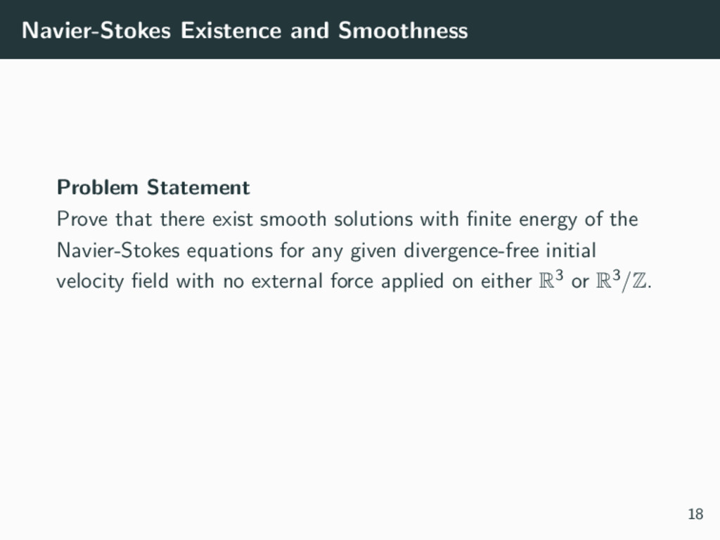
smooth solutions with finite energy of the Navier-Stokes equations for any given divergence-free initial velocity field with no external force applied on either R3 or R3/Z. 18
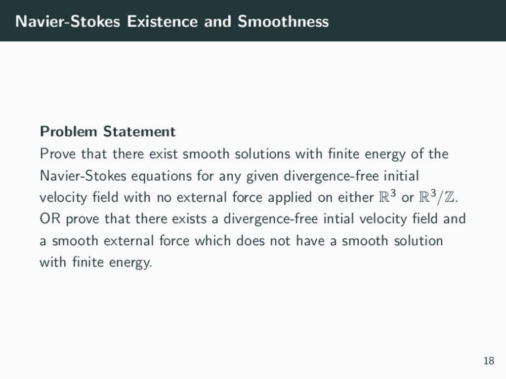
smooth solutions with finite energy of the Navier-Stokes equations for any given divergence-free initial velocity field with no external force applied on either R3 or R3/Z. OR prove that there exists a divergence-free intial velocity field and a smooth external force which does not have a smooth solution with finite energy. 18
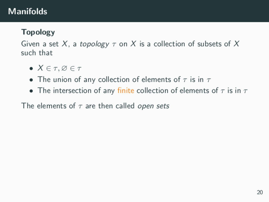
X is a collection of subsets of X such that • X ∈ τ, ∅ ∈ τ • The union of any collection of elements of τ is in τ • The intersection of any finite collection of elements of τ is in τ The elements of τ are then called open sets 20
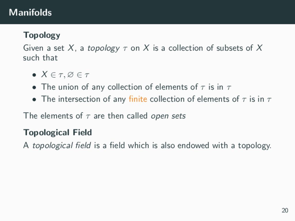
X is a collection of subsets of X such that • X ∈ τ, ∅ ∈ τ • The union of any collection of elements of τ is in τ • The intersection of any finite collection of elements of τ is in τ The elements of τ are then called open sets Topological Field A topological field is a field which is also endowed with a topology. 20
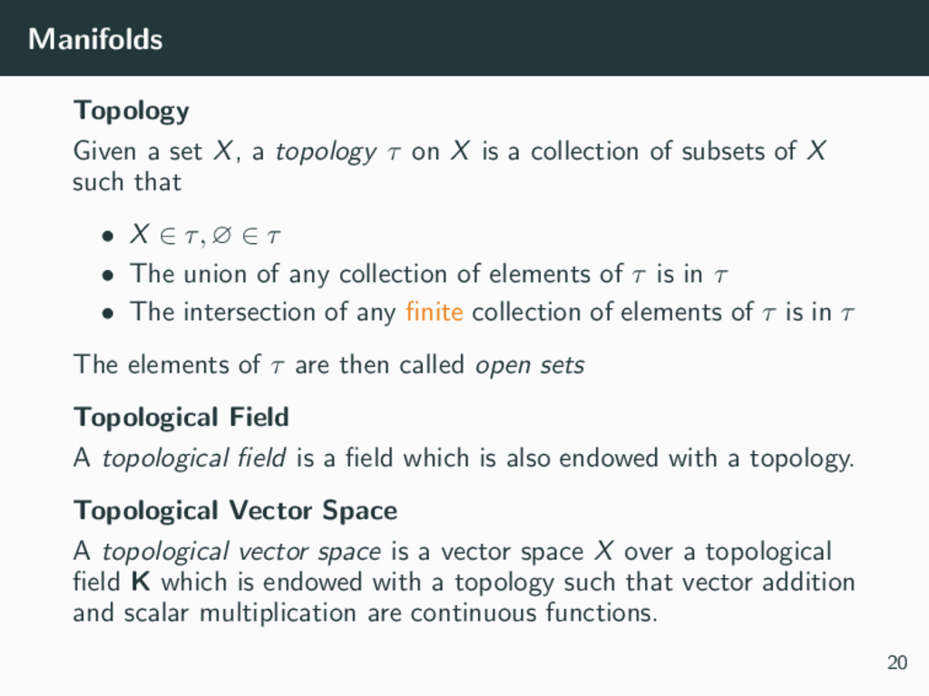
X is a collection of subsets of X such that • X ∈ τ, ∅ ∈ τ • The union of any collection of elements of τ is in τ • The intersection of any finite collection of elements of τ is in τ The elements of τ are then called open sets Topological Field A topological field is a field which is also endowed with a topology. Topological Vector Space A topological vector space is a vector space X over a topological field K which is endowed with a topology such that vector addition and scalar multiplication are continuous functions. 20
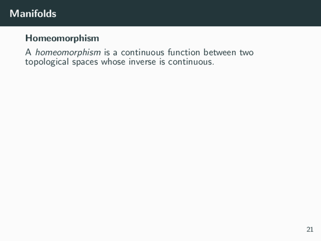
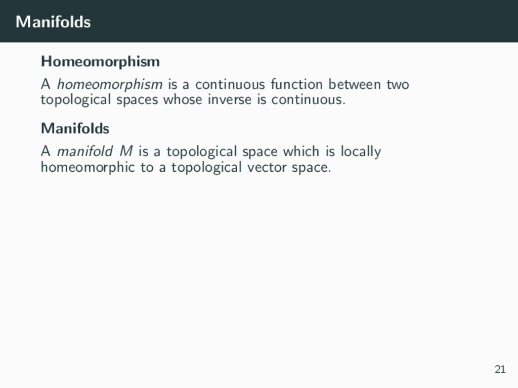
topological spaces whose inverse is continuous. Manifolds A manifold M is a topological space which is locally homeomorphic to a topological vector space. 21
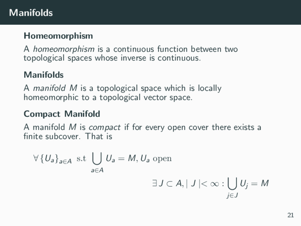
topological spaces whose inverse is continuous. Manifolds A manifold M is a topological space which is locally homeomorphic to a topological vector space. Compact Manifold A manifold M is compact if for every open cover there exists a finite subcover. That is ∀ {Ua}a∈A s.t a∈A Ua = M, Ua open ∃ J ⊂ A, | J |< ∞ : j∈J Uj = M 21
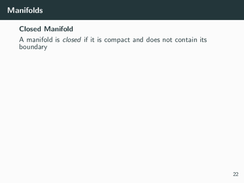
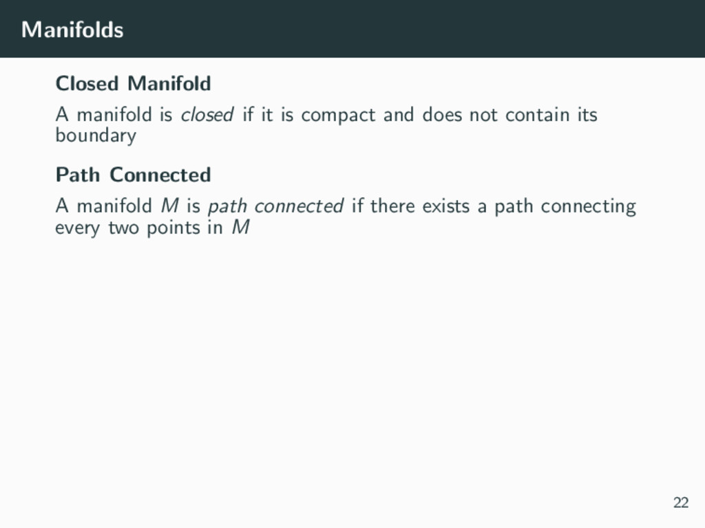
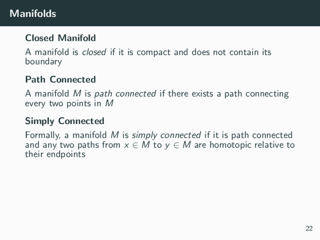
compact and does not contain its boundary Path Connected A manifold M is path connected if there exists a path connecting every two points in M Simply Connected Formally, a manifold M is simply connected if it is path connected and any two paths from x ∈ M to y ∈ M are homotopic relative to their endpoints 22
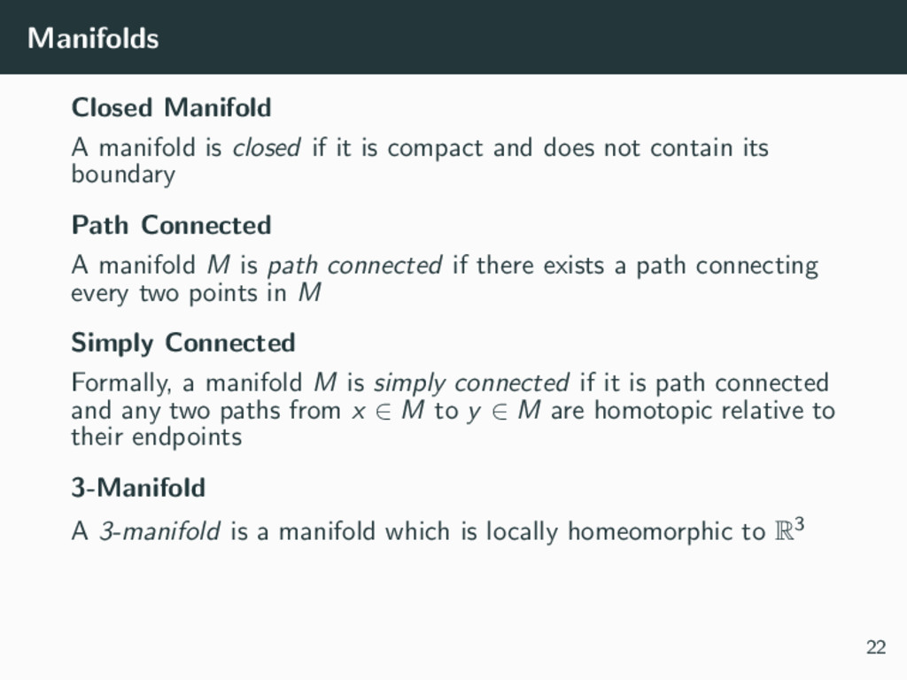
compact and does not contain its boundary Path Connected A manifold M is path connected if there exists a path connecting every two points in M Simply Connected Formally, a manifold M is simply connected if it is path connected and any two paths from x ∈ M to y ∈ M are homotopic relative to their endpoints 3-Manifold A 3-manifold is a manifold which is locally homeomorphic to R3 22
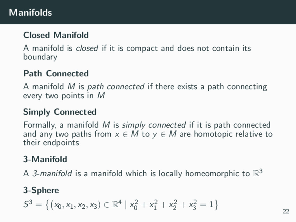
compact and does not contain its boundary Path Connected A manifold M is path connected if there exists a path connecting every two points in M Simply Connected Formally, a manifold M is simply connected if it is path connected and any two paths from x ∈ M to y ∈ M are homotopic relative to their endpoints 3-Manifold A 3-manifold is a manifold which is locally homeomorphic to R3 3-Sphere S3 = x0, x1, x2, x3) ∈ R4 | x2 0 + x2 1 + x2 2 + x2 3 = 1 22
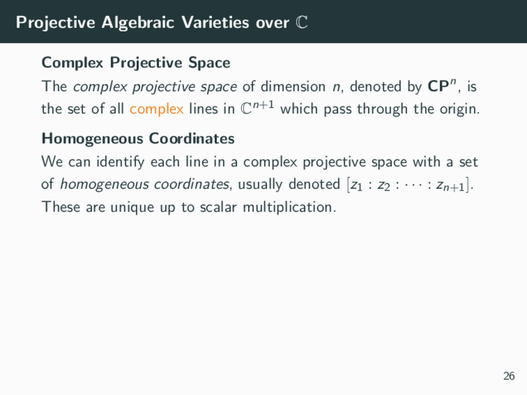
projective space of dimension n, denoted by CPn, is the set of all complex lines in Cn+1 which pass through the origin. Homogeneous Coordinates We can identify each line in a complex projective space with a set of homogeneous coordinates, usually denoted [z1 : z2 : · · · : zn+1]. These are unique up to scalar multiplication. 26
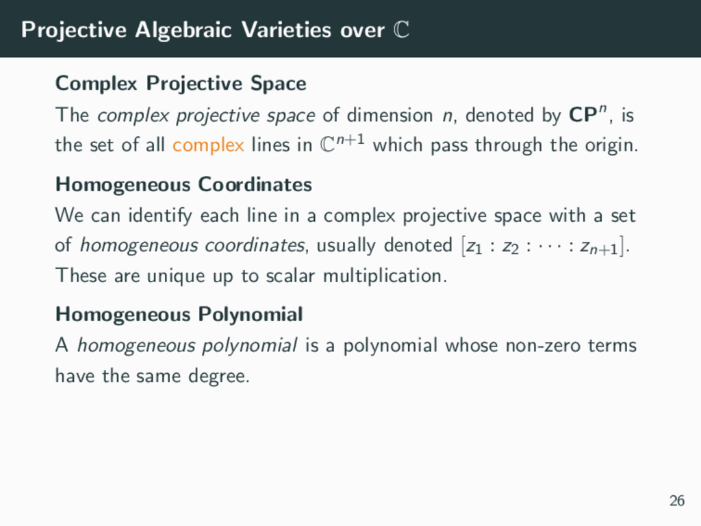
projective space of dimension n, denoted by CPn, is the set of all complex lines in Cn+1 which pass through the origin. Homogeneous Coordinates We can identify each line in a complex projective space with a set of homogeneous coordinates, usually denoted [z1 : z2 : · · · : zn+1]. These are unique up to scalar multiplication. Homogeneous Polynomial A homogeneous polynomial is a polynomial whose non-zero terms have the same degree. 26
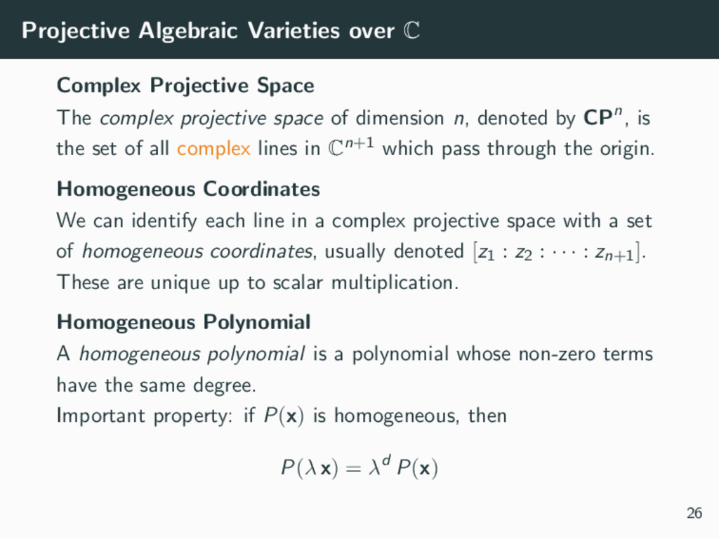
projective space of dimension n, denoted by CPn, is the set of all complex lines in Cn+1 which pass through the origin. Homogeneous Coordinates We can identify each line in a complex projective space with a set of homogeneous coordinates, usually denoted [z1 : z2 : · · · : zn+1]. These are unique up to scalar multiplication. Homogeneous Polynomial A homogeneous polynomial is a polynomial whose non-zero terms have the same degree. Important property: if P(x) is homogeneous, then P(λ x) = λd P(x) 26
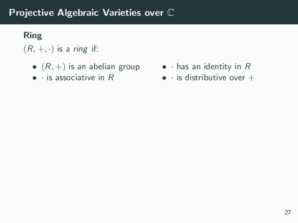
a ring if: • (R, +) is an abelian group • · is associative in R • · has an identity in R • · is distributive over + Ideal Let (R, +, ·) be a ring. Then I ⊆ R is an ideal if: • (I, +) ≤ (R, +) • ∀ i ∈ I, ∀ r ∈ R, i ·r, r ·i ∈ I 27
a ring if: • (R, +) is an abelian group • · is associative in R • · has an identity in R • · is distributive over + Ideal Let (R, +, ·) be a ring. Then I ⊆ R is an ideal if: • (I, +) ≤ (R, +) • ∀ i ∈ I, ∀ r ∈ R, i ·r, r ·i ∈ I Prime Ideal An ideal (P, +, ·) with P ⊂ R is a prime ideal if a, b ∈ R, a · b ∈ P ⇒ a ∈ P or b ∈ P 27
of a set of homogeneous polynomials S in CPn is defined to be Z(S) = {x ∈ CPn | f (x) = 0 ∀ f ∈ S} Projective Algebraic Variety A projective algebraic variety is a zero locus of a set of homogeneous polynomials which form a prime ideal 28
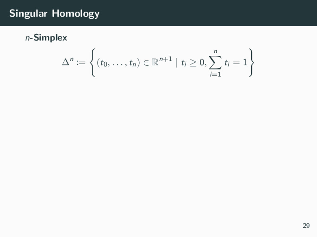
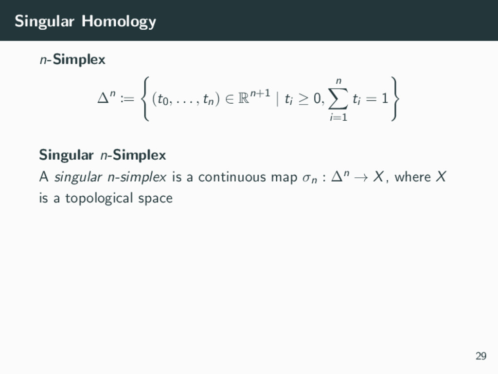
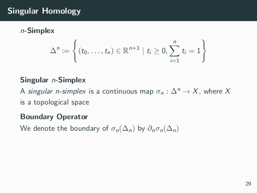
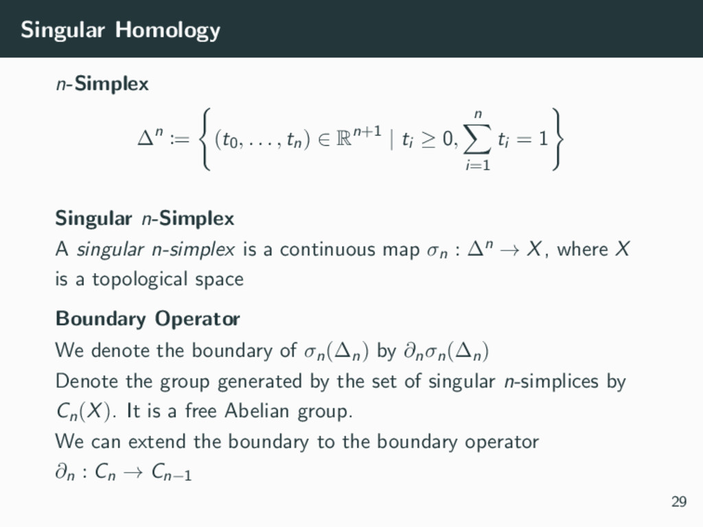
tn) ∈ Rn+1 | ti ≥ 0, n i=1 ti = 1 Singular n-Simplex A singular n-simplex is a continuous map σn : ∆n → X, where X is a topological space Boundary Operator We denote the boundary of σn(∆n) by ∂nσn(∆n) 29
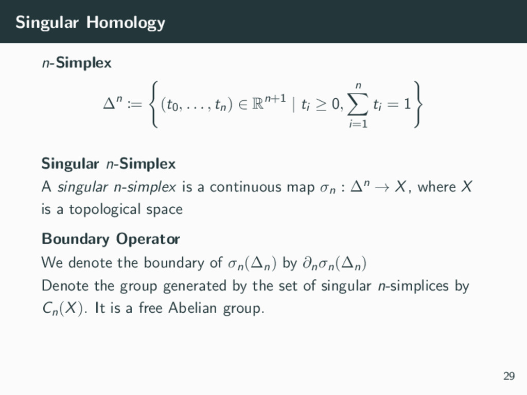
tn) ∈ Rn+1 | ti ≥ 0, n i=1 ti = 1 Singular n-Simplex A singular n-simplex is a continuous map σn : ∆n → X, where X is a topological space Boundary Operator We denote the boundary of σn(∆n) by ∂nσn(∆n) Denote the group generated by the set of singular n-simplices by Cn(X). It is a free Abelian group. 29
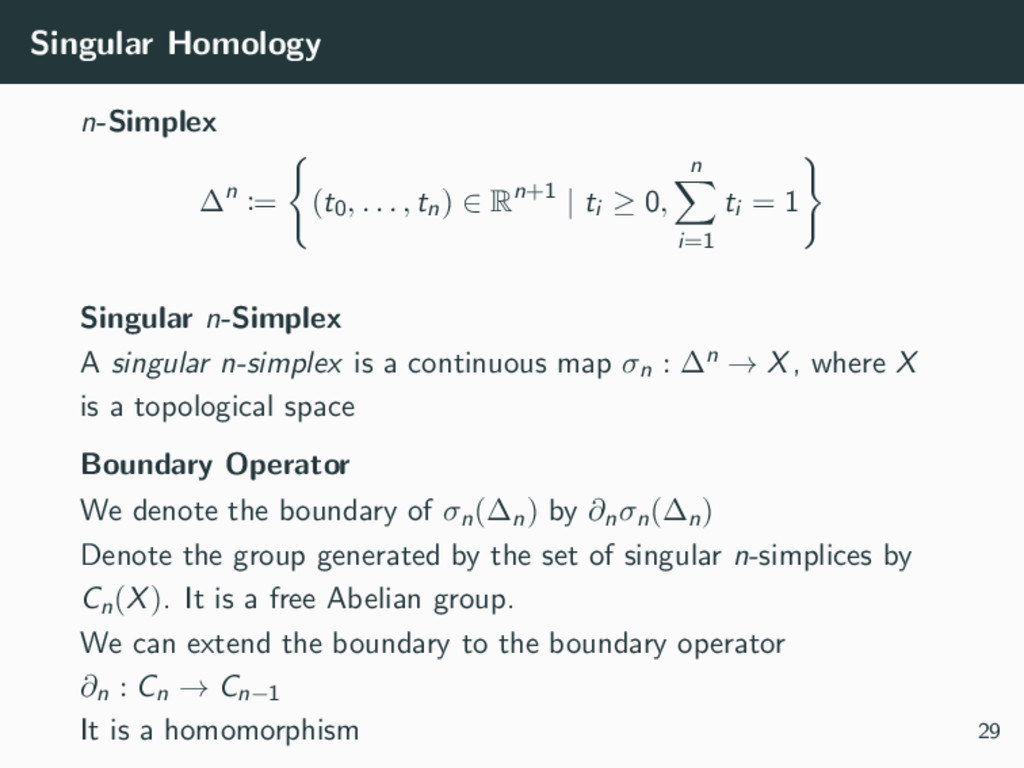
tn) ∈ Rn+1 | ti ≥ 0, n i=1 ti = 1 Singular n-Simplex A singular n-simplex is a continuous map σn : ∆n → X, where X is a topological space Boundary Operator We denote the boundary of σn(∆n) by ∂nσn(∆n) Denote the group generated by the set of singular n-simplices by Cn(X). It is a free Abelian group. We can extend the boundary to the boundary operator ∂n : Cn → Cn−1 29
tn) ∈ Rn+1 | ti ≥ 0, n i=1 ti = 1 Singular n-Simplex A singular n-simplex is a continuous map σn : ∆n → X, where X is a topological space Boundary Operator We denote the boundary of σn(∆n) by ∂nσn(∆n) Denote the group generated by the set of singular n-simplices by Cn(X). It is a free Abelian group. We can extend the boundary to the boundary operator ∂n : Cn → Cn−1 It is a homomorphism 29
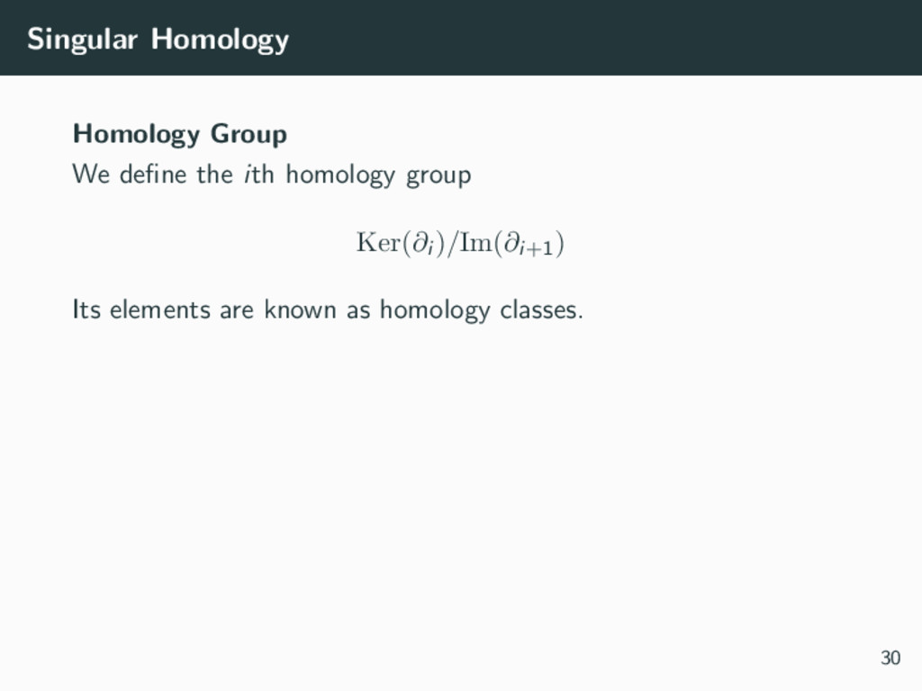
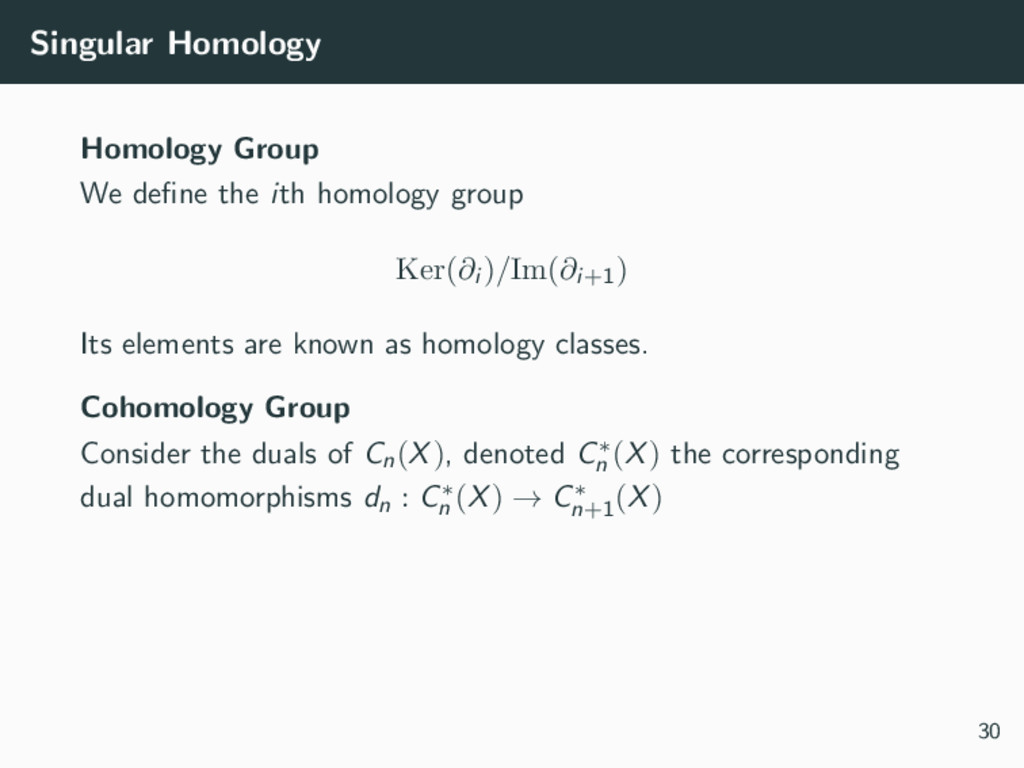
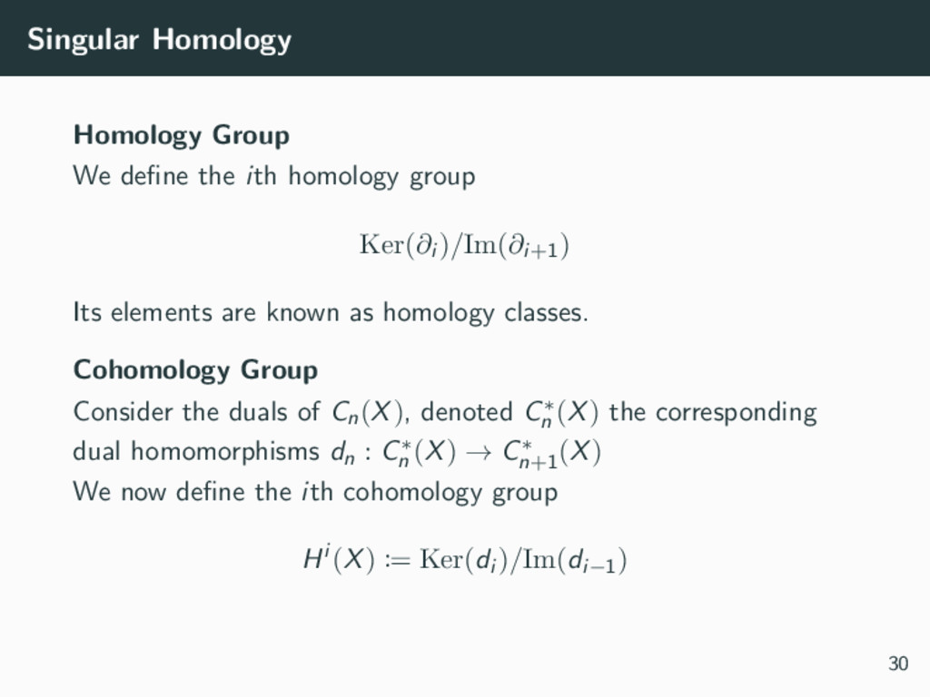
Ker(∂i )/Im(∂i+1) Its elements are known as homology classes. Cohomology Group Consider the duals of Cn(X), denoted C∗ n (X) the corresponding dual homomorphisms dn : C∗ n (X) → C∗ n+1 (X) 30
Ker(∂i )/Im(∂i+1) Its elements are known as homology classes. Cohomology Group Consider the duals of Cn(X), denoted C∗ n (X) the corresponding dual homomorphisms dn : C∗ n (X) → C∗ n+1 (X) We now define the ith cohomology group Hi (X) := Ker(di )/Im(di−1) 30
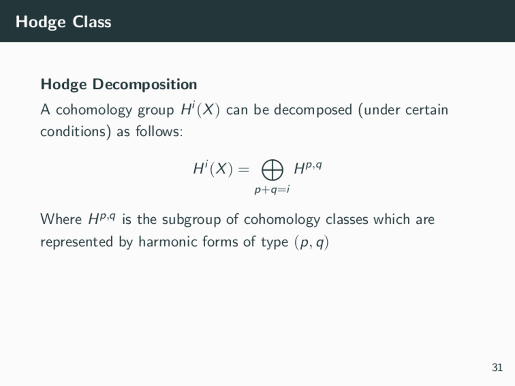
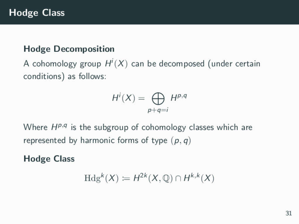
be decomposed (under certain conditions) as follows: Hi (X) = p+q=i Hp,q Where Hp,q is the subgroup of cohomology classes which are represented by harmonic forms of type (p, q) 31
be decomposed (under certain conditions) as follows: Hi (X) = p+q=i Hp,q Where Hp,q is the subgroup of cohomology classes which are represented by harmonic forms of type (p, q) Hodge Class Hdgk(X) := H2k(X, Q) ∩ Hk,k(X) 31
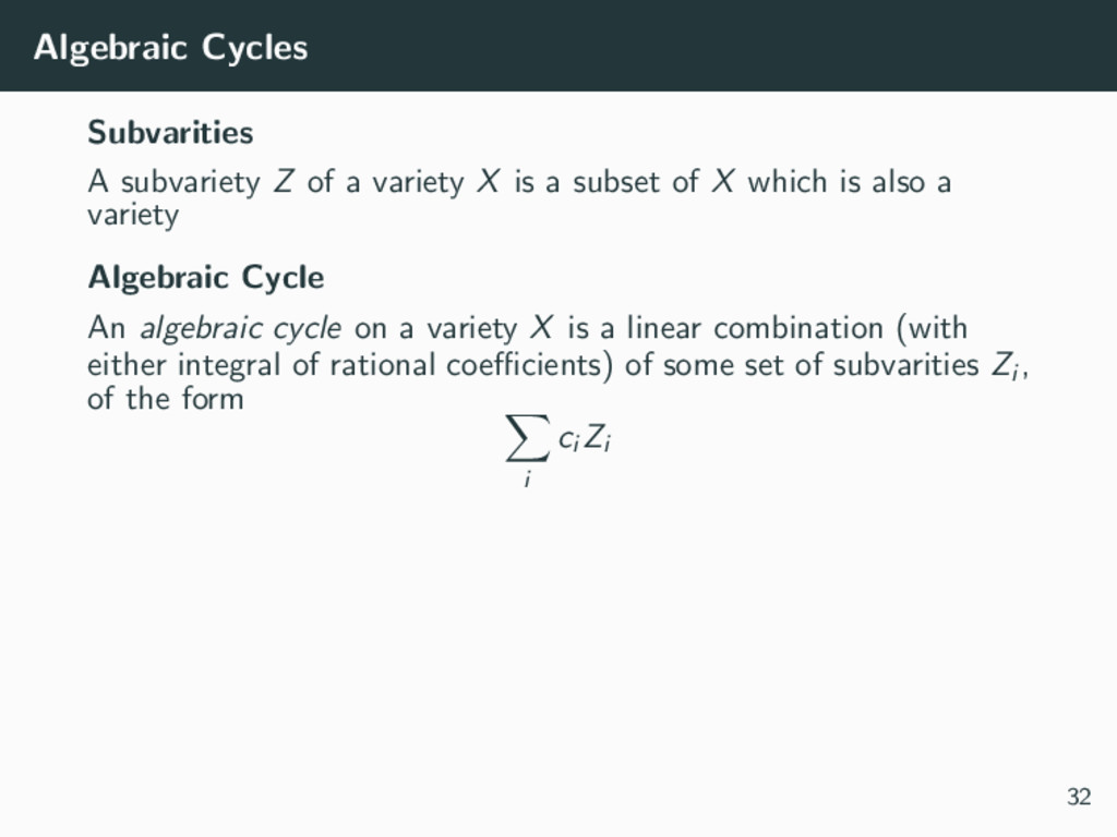
is a subset of X which is also a variety Algebraic Cycle An algebraic cycle on a variety X is a linear combination (with either integral of rational coefficients) of some set of subvarities Zi , of the form i ci Zi 32
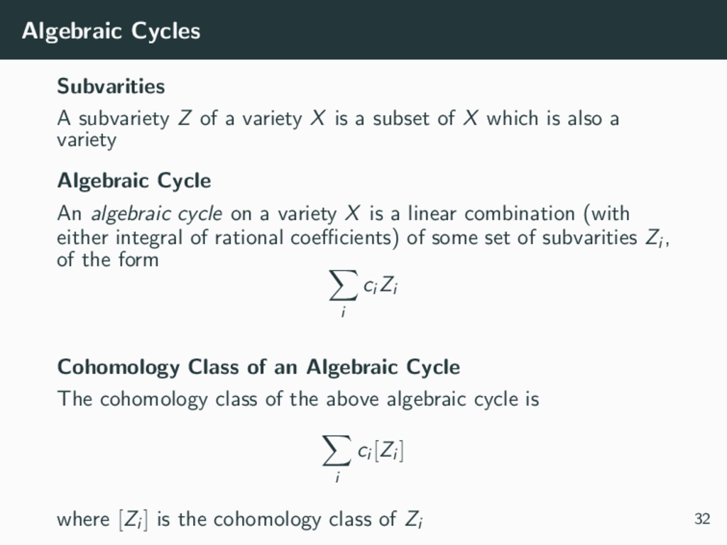
is a subset of X which is also a variety Algebraic Cycle An algebraic cycle on a variety X is a linear combination (with either integral of rational coefficients) of some set of subvarities Zi , of the form i ci Zi Cohomology Class of an Algebraic Cycle The cohomology class of the above algebraic cycle is i ci [Zi ] where [Zi ] is the cohomology class of Zi 32
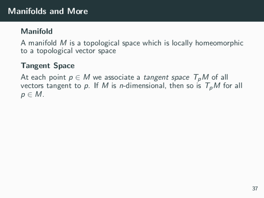
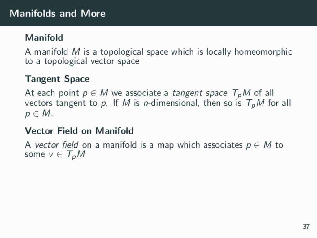
space which is locally homeomorphic to a topological vector space Tangent Space At each point p ∈ M we associate a tangent space TpM of all vectors tangent to p. If M is n-dimensional, then so is TpM for all p ∈ M. 37
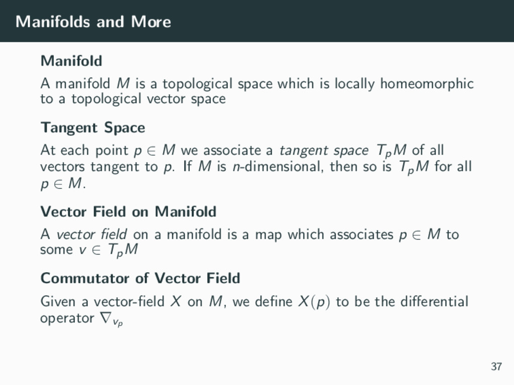
space which is locally homeomorphic to a topological vector space Tangent Space At each point p ∈ M we associate a tangent space TpM of all vectors tangent to p. If M is n-dimensional, then so is TpM for all p ∈ M. Vector Field on Manifold A vector field on a manifold is a map which associates p ∈ M to some v ∈ TpM 37
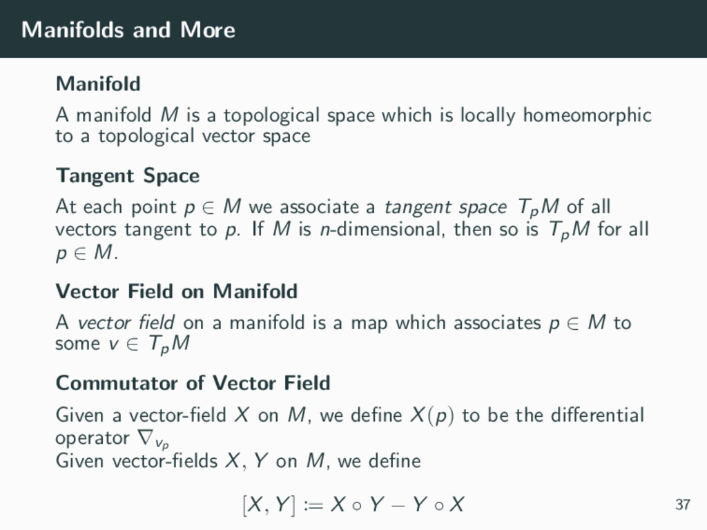
space which is locally homeomorphic to a topological vector space Tangent Space At each point p ∈ M we associate a tangent space TpM of all vectors tangent to p. If M is n-dimensional, then so is TpM for all p ∈ M. Vector Field on Manifold A vector field on a manifold is a map which associates p ∈ M to some v ∈ TpM Commutator of Vector Field Given a vector-field X on M, we define X(p) to be the differential operator ∇vp 37
space which is locally homeomorphic to a topological vector space Tangent Space At each point p ∈ M we associate a tangent space TpM of all vectors tangent to p. If M is n-dimensional, then so is TpM for all p ∈ M. Vector Field on Manifold A vector field on a manifold is a map which associates p ∈ M to some v ∈ TpM Commutator of Vector Field Given a vector-field X on M, we define X(p) to be the differential operator ∇vp Given vector-fields X, Y on M, we define [X, Y ] := X ◦ Y − Y ◦ X 37
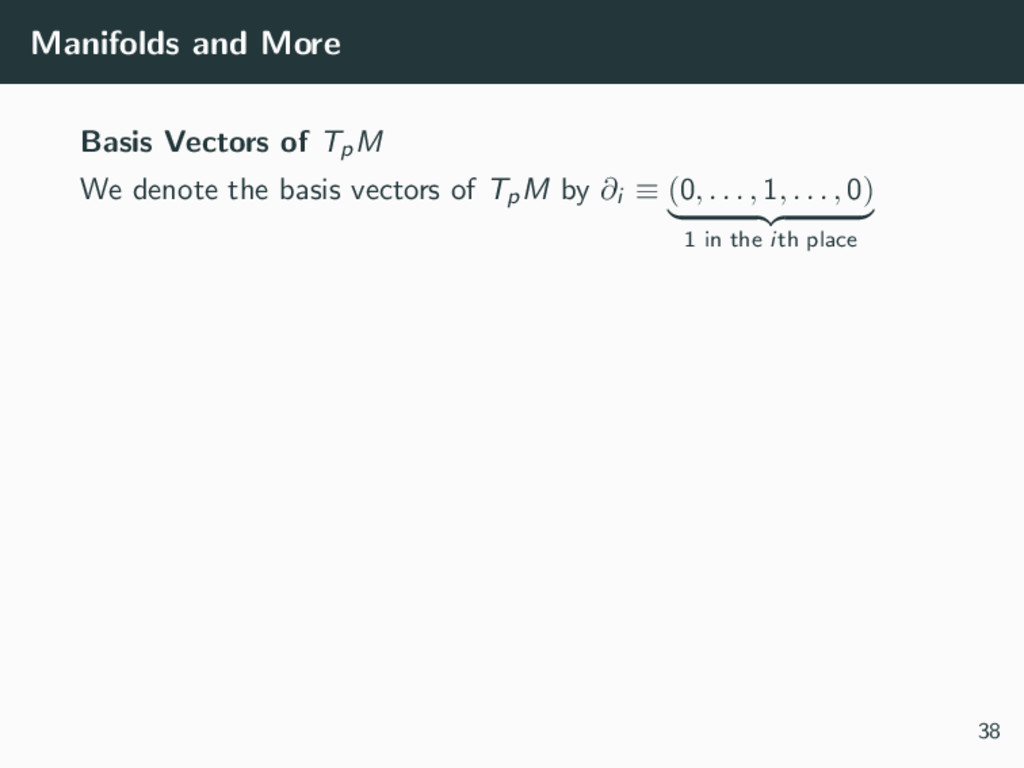
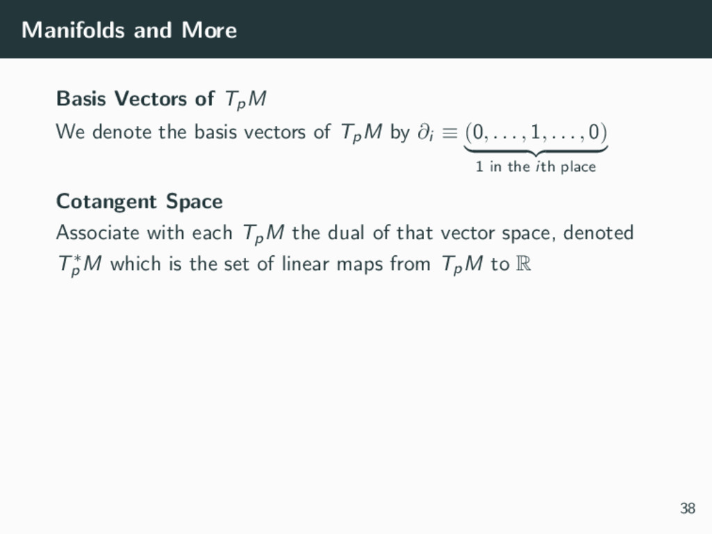
basis vectors of TpM by ∂i ≡ (0, . . . , 1, . . . , 0) 1 in the ith place Cotangent Space Associate with each TpM the dual of that vector space, denoted T∗ p M which is the set of linear maps from TpM to R 38
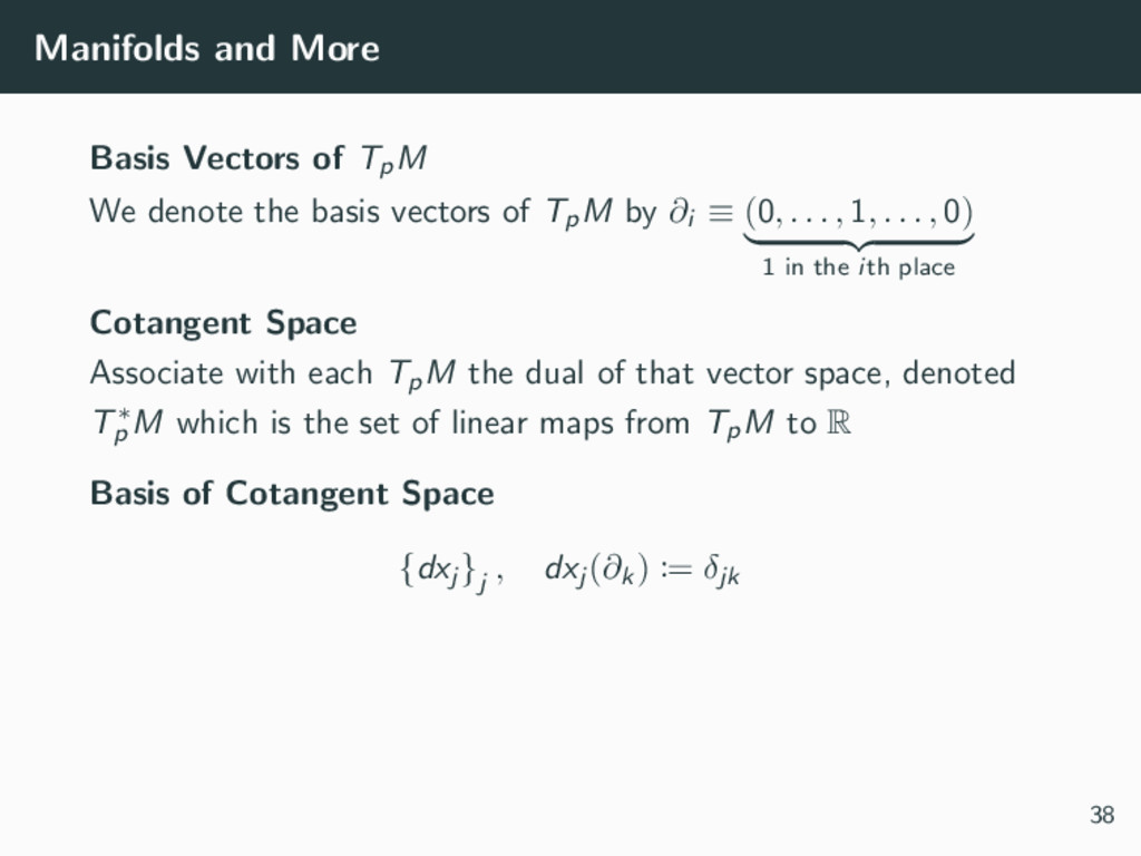
basis vectors of TpM by ∂i ≡ (0, . . . , 1, . . . , 0) 1 in the ith place Cotangent Space Associate with each TpM the dual of that vector space, denoted T∗ p M which is the set of linear maps from TpM to R Basis of Cotangent Space {dxj } j , dxj (∂k) := δjk 38
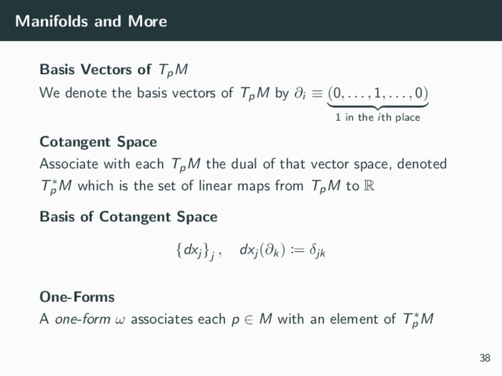
basis vectors of TpM by ∂i ≡ (0, . . . , 1, . . . , 0) 1 in the ith place Cotangent Space Associate with each TpM the dual of that vector space, denoted T∗ p M which is the set of linear maps from TpM to R Basis of Cotangent Space {dxj } j , dxj (∂k) := δjk One-Forms A one-form ω associates each p ∈ M with an element of T∗ p M 38
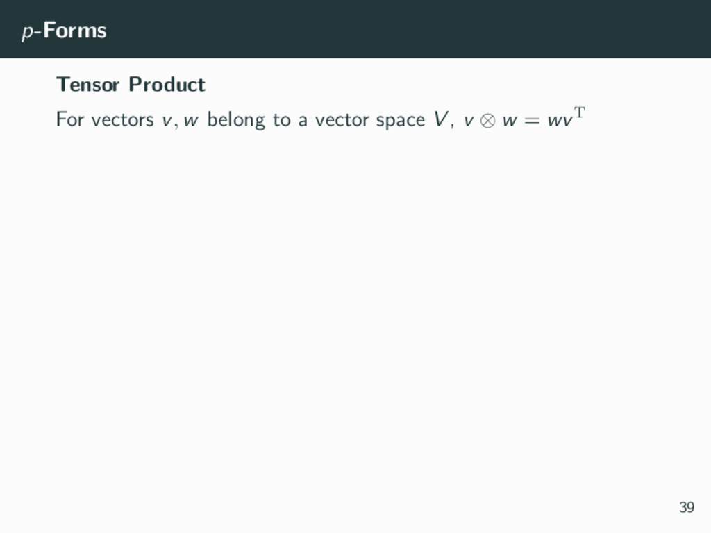
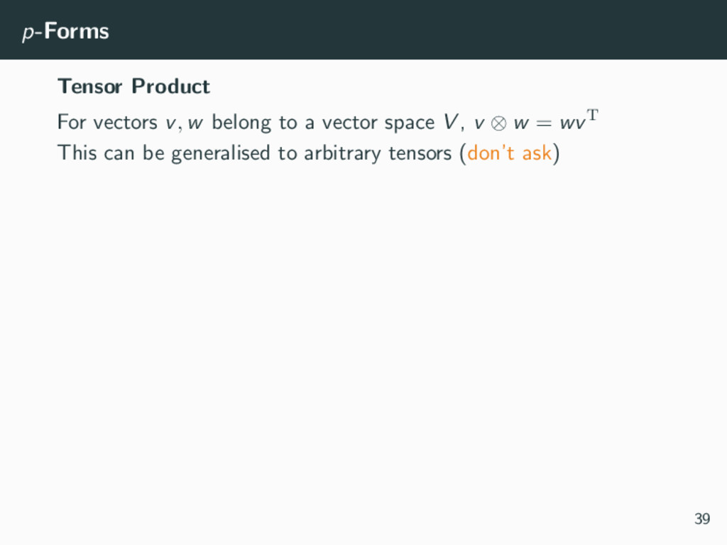
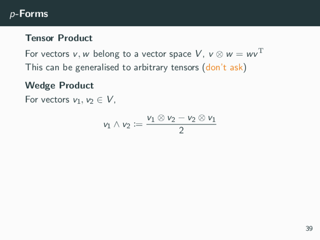
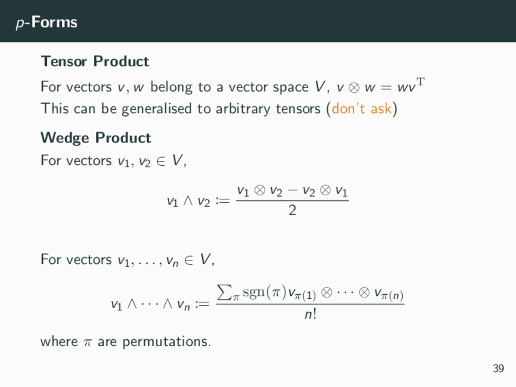
vector space V , v ⊗ w = wvT This can be generalised to arbitrary tensors (don’t ask) Wedge Product For vectors v1, v2 ∈ V , v1 ∧ v2 := v1 ⊗ v2 − v2 ⊗ v1 2 39
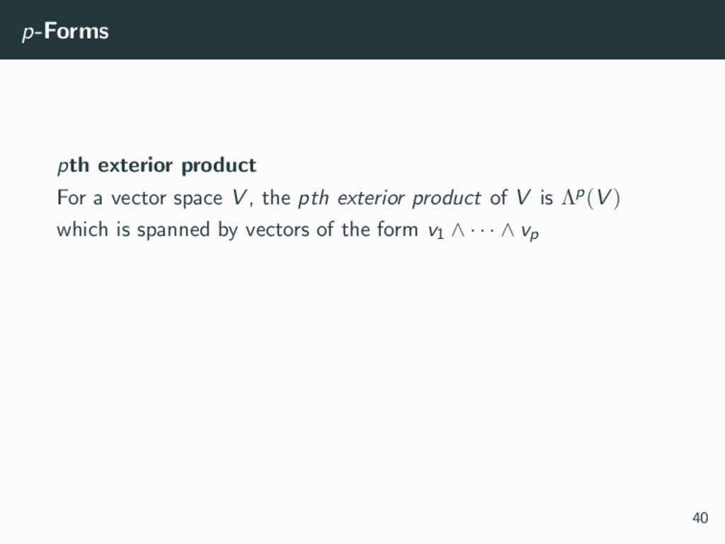
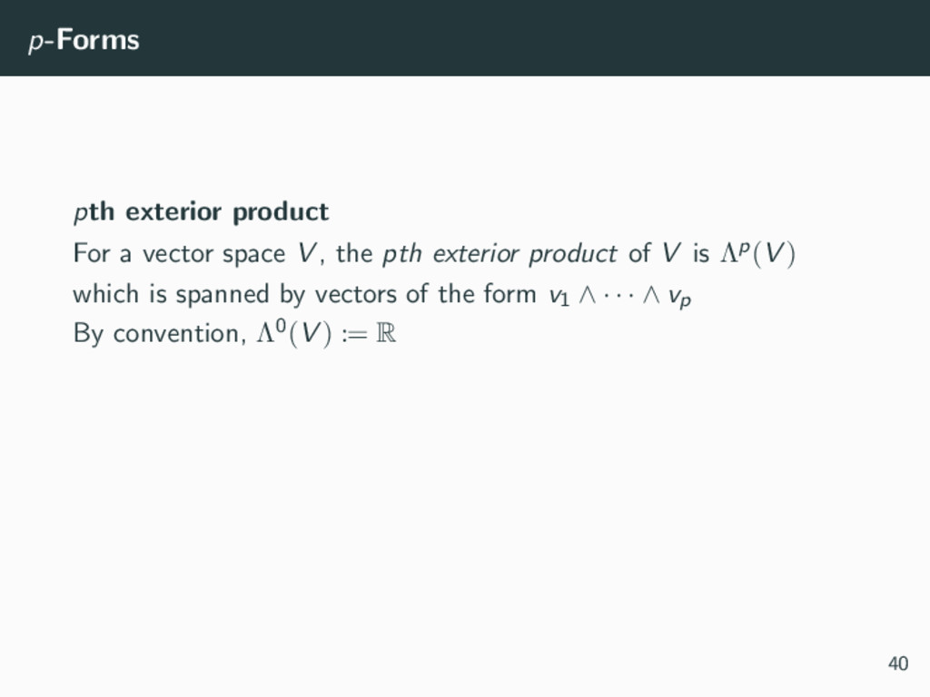
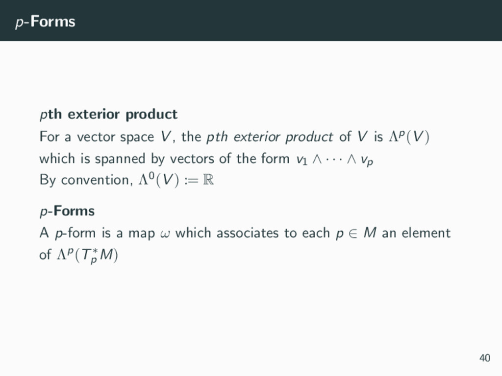
the pth exterior product of V is Λp(V ) which is spanned by vectors of the form v1 ∧ · · · ∧ vp By convention, Λ0(V ) := R p-Forms A p-form is a map ω which associates to each p ∈ M an element of Λp(T∗ p M) 40
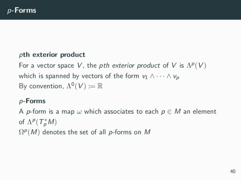
the pth exterior product of V is Λp(V ) which is spanned by vectors of the form v1 ∧ · · · ∧ vp By convention, Λ0(V ) := R p-Forms A p-form is a map ω which associates to each p ∈ M an element of Λp(T∗ p M) Ωp(M) denotes the set of all p-forms on M 40
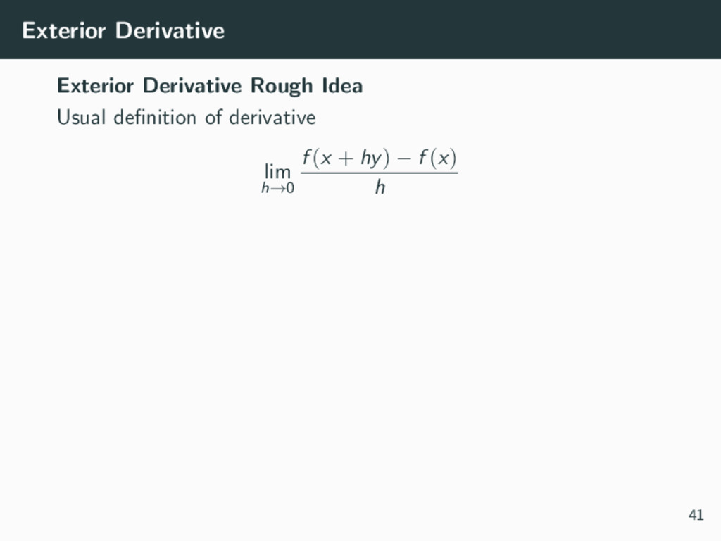
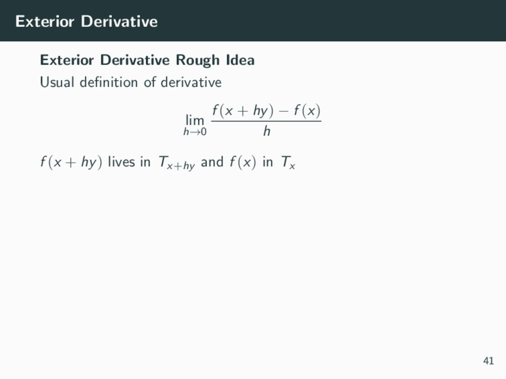
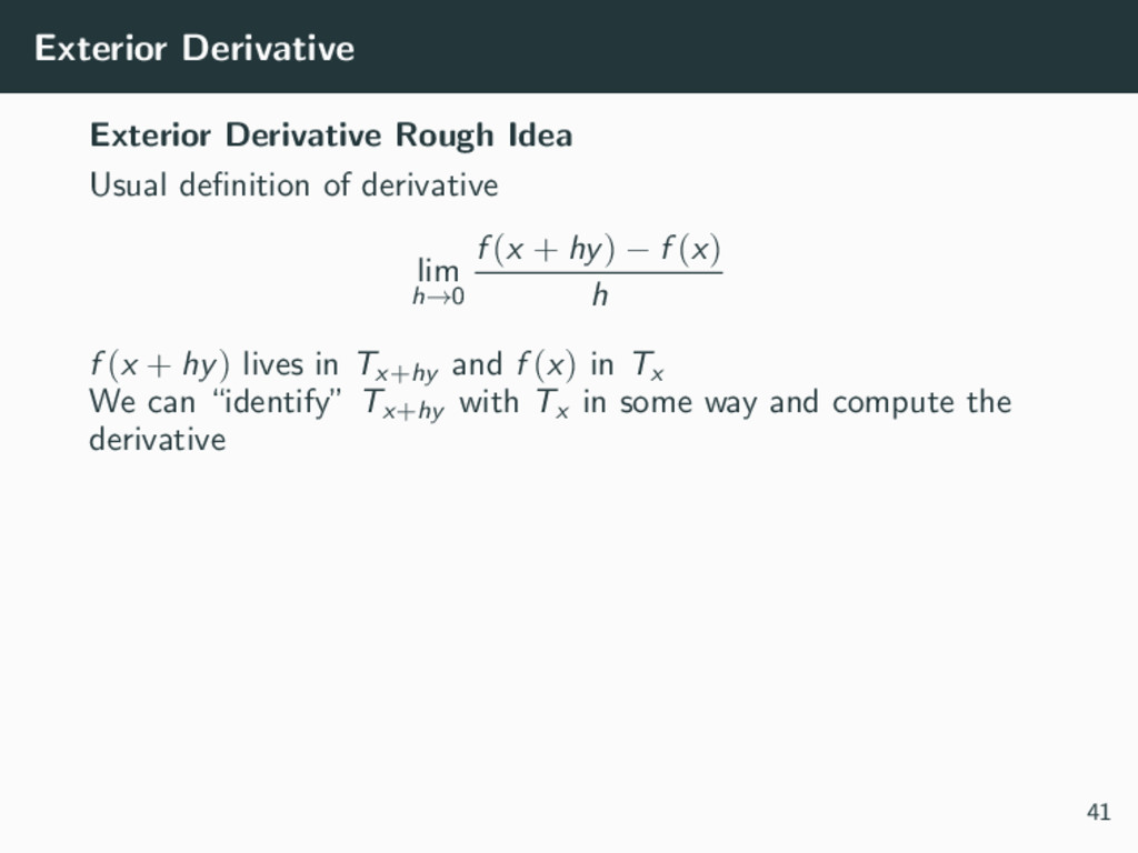
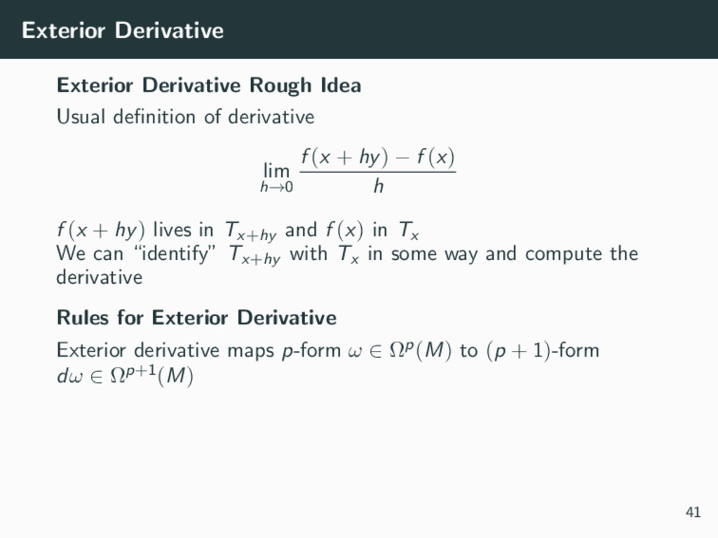
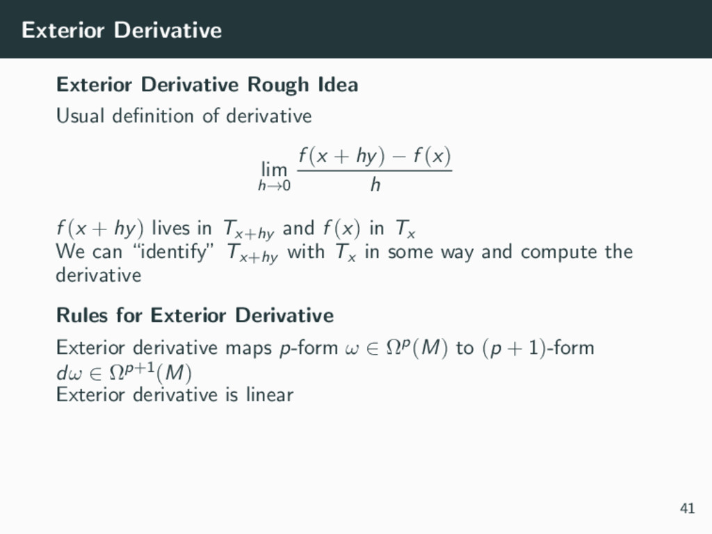
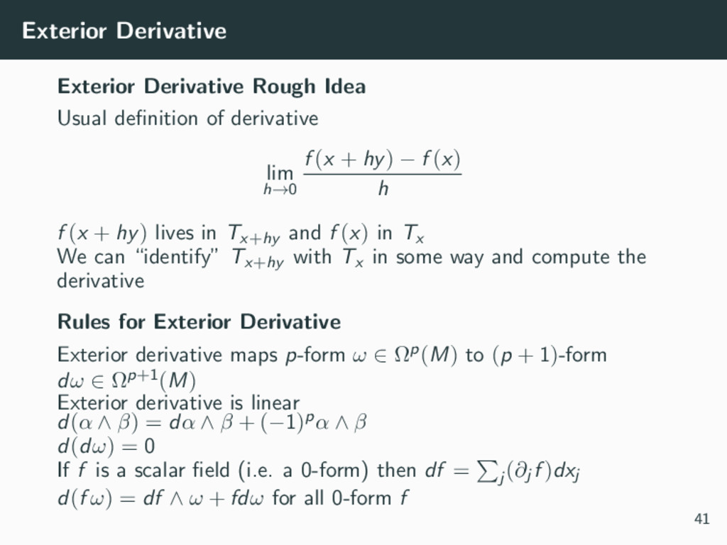
lim h→0 f (x + hy) − f (x) h f (x + hy) lives in Tx+hy and f (x) in Tx We can “identify” Tx+hy with Tx in some way and compute the derivative Rules for Exterior Derivative Exterior derivative maps p-form ω ∈ Ωp(M) to (p + 1)-form dω ∈ Ωp+1(M) 41
lim h→0 f (x + hy) − f (x) h f (x + hy) lives in Tx+hy and f (x) in Tx We can “identify” Tx+hy with Tx in some way and compute the derivative Rules for Exterior Derivative Exterior derivative maps p-form ω ∈ Ωp(M) to (p + 1)-form dω ∈ Ωp+1(M) Exterior derivative is linear 41
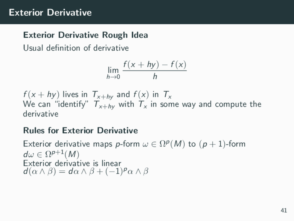
lim h→0 f (x + hy) − f (x) h f (x + hy) lives in Tx+hy and f (x) in Tx We can “identify” Tx+hy with Tx in some way and compute the derivative Rules for Exterior Derivative Exterior derivative maps p-form ω ∈ Ωp(M) to (p + 1)-form dω ∈ Ωp+1(M) Exterior derivative is linear d(α ∧ β) = dα ∧ β + (−1)pα ∧ β 41
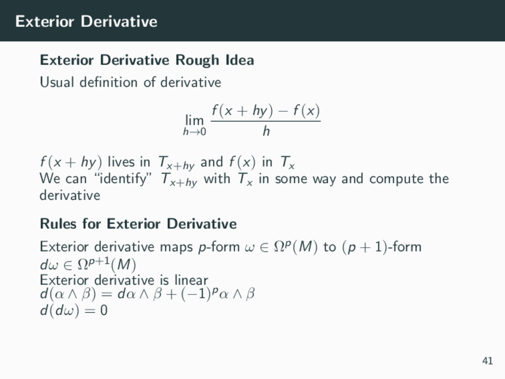
lim h→0 f (x + hy) − f (x) h f (x + hy) lives in Tx+hy and f (x) in Tx We can “identify” Tx+hy with Tx in some way and compute the derivative Rules for Exterior Derivative Exterior derivative maps p-form ω ∈ Ωp(M) to (p + 1)-form dω ∈ Ωp+1(M) Exterior derivative is linear d(α ∧ β) = dα ∧ β + (−1)pα ∧ β d(dω) = 0 41
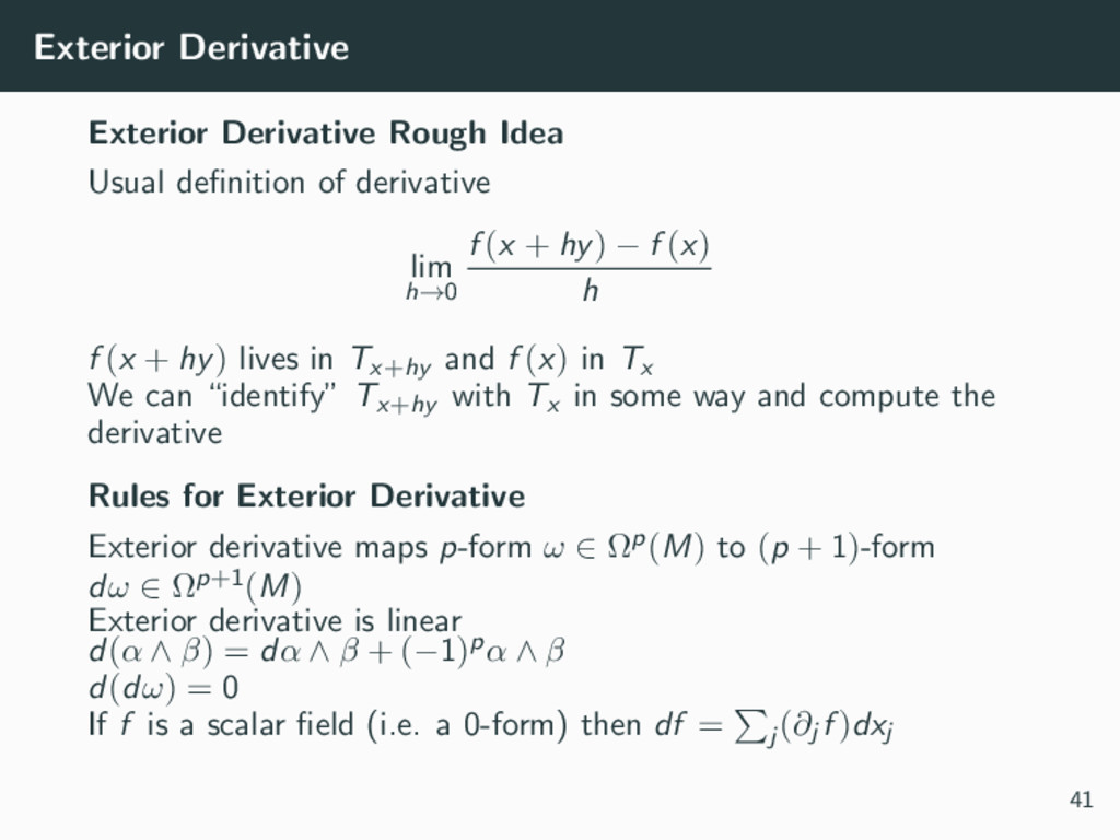
lim h→0 f (x + hy) − f (x) h f (x + hy) lives in Tx+hy and f (x) in Tx We can “identify” Tx+hy with Tx in some way and compute the derivative Rules for Exterior Derivative Exterior derivative maps p-form ω ∈ Ωp(M) to (p + 1)-form dω ∈ Ωp+1(M) Exterior derivative is linear d(α ∧ β) = dα ∧ β + (−1)pα ∧ β d(dω) = 0 If f is a scalar field (i.e. a 0-form) then df = j (∂j f )dxj 41
lim h→0 f (x + hy) − f (x) h f (x + hy) lives in Tx+hy and f (x) in Tx We can “identify” Tx+hy with Tx in some way and compute the derivative Rules for Exterior Derivative Exterior derivative maps p-form ω ∈ Ωp(M) to (p + 1)-form dω ∈ Ωp+1(M) Exterior derivative is linear d(α ∧ β) = dα ∧ β + (−1)pα ∧ β d(dω) = 0 If f is a scalar field (i.e. a 0-form) then df = j (∂j f )dxj d(f ω) = df ∧ ω + fdω for all 0-form f 41
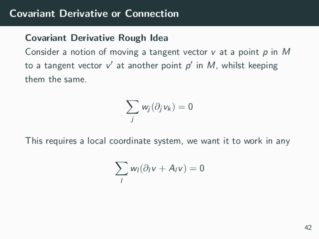
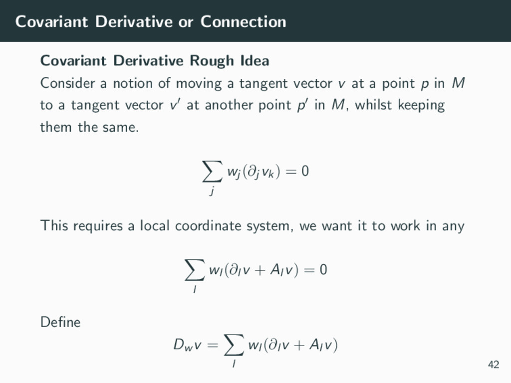
notion of moving a tangent vector v at a point p in M to a tangent vector v at another point p in M, whilst keeping them the same. j wj (∂j vk) = 0 This requires a local coordinate system, we want it to work in any 42
notion of moving a tangent vector v at a point p in M to a tangent vector v at another point p in M, whilst keeping them the same. j wj (∂j vk) = 0 This requires a local coordinate system, we want it to work in any l wl (∂l v + Al v) = 0 42
notion of moving a tangent vector v at a point p in M to a tangent vector v at another point p in M, whilst keeping them the same. j wj (∂j vk) = 0 This requires a local coordinate system, we want it to work in any l wl (∂l v + Al v) = 0 Define Dw v = l wl (∂l v + Al v) 42
vector space to each point in the manifold. Denote it Vp and we call it a fibre. M plus the Vps are called a vector bundle. (All fibres must have the same dimension) 43
vector space to each point in the manifold. Denote it Vp and we call it a fibre. M plus the Vps are called a vector bundle. (All fibres must have the same dimension) Sections A section is a map s which associates an element of Vp to each p ∈ M 43
vector space to each point in the manifold. Denote it Vp and we call it a fibre. M plus the Vps are called a vector bundle. (All fibres must have the same dimension) Sections A section is a map s which associates an element of Vp to each p ∈ M Covariant Derivative We can extend the covariant derivative to work on arbitrary sections in an analogous way 43
of it V , define a bundle over a manifold M where each fibre is V . Sections of a G-Bundle A section of this G-bundle assigns to each p ∈ M a group element g(p) acting on V . 44
of it V , define a bundle over a manifold M where each fibre is V . Sections of a G-Bundle A section of this G-bundle assigns to each p ∈ M a group element g(p) acting on V . Gauge Symmetries and Groups We call g a gauge transformation or gauge symmetry and G the gauge group. 44
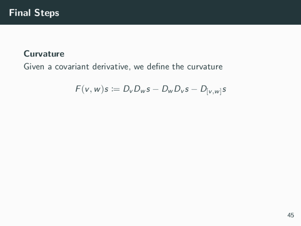
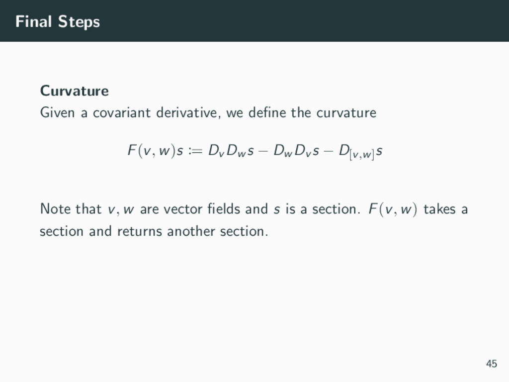
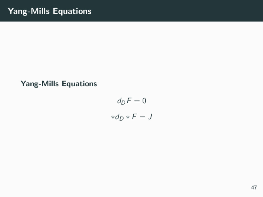
curvature F(v, w)s := Dv Dw s − Dw Dv s − D[v,w] s Note that v, w are vector fields and s is a section. F(v, w) takes a section and returns another section. 45
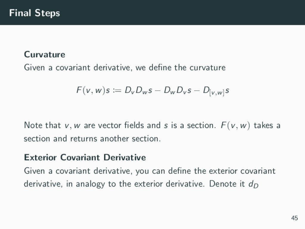
curvature F(v, w)s := Dv Dw s − Dw Dv s − D[v,w] s Note that v, w are vector fields and s is a section. F(v, w) takes a section and returns another section. Exterior Covariant Derivative Given a covariant derivative, you can define the exterior covariant derivative, in analogy to the exterior derivative. Denote it dD 45
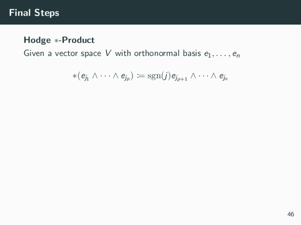
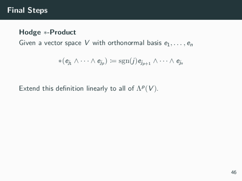
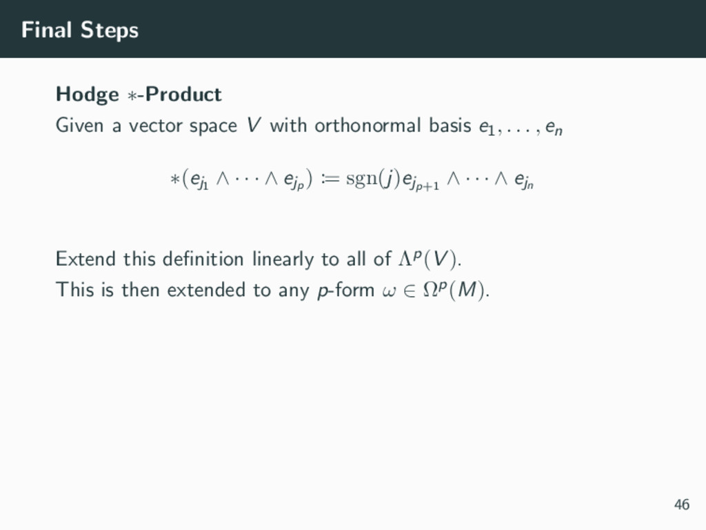
orthonormal basis e1, . . . , en ∗(ej1 ∧ · · · ∧ ejp ) := sgn(j)ejp+1 ∧ · · · ∧ ejn Extend this definition linearly to all of Λp(V ). This is then extended to any p-form ω ∈ Ωp(M). 46
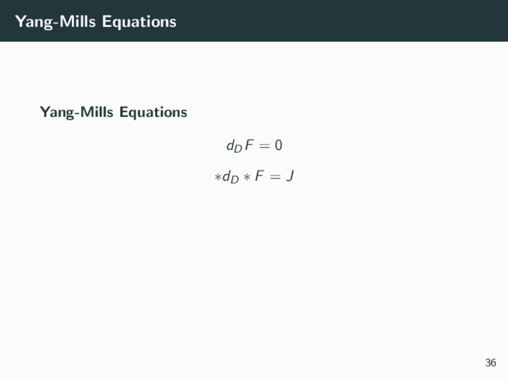
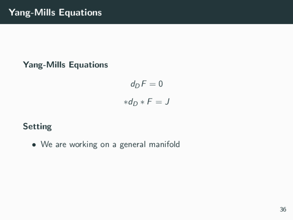
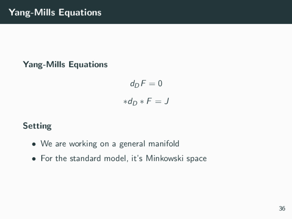
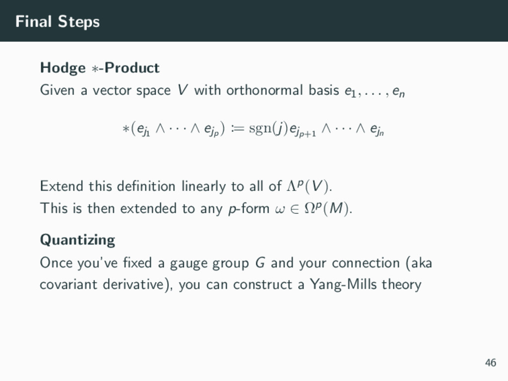
orthonormal basis e1, . . . , en ∗(ej1 ∧ · · · ∧ ejp ) := sgn(j)ejp+1 ∧ · · · ∧ ejn Extend this definition linearly to all of Λp(V ). This is then extended to any p-form ω ∈ Ωp(M). Quantizing Once you’ve fixed a gauge group G and your connection (aka covariant derivative), you can construct a Yang-Mills theory 46
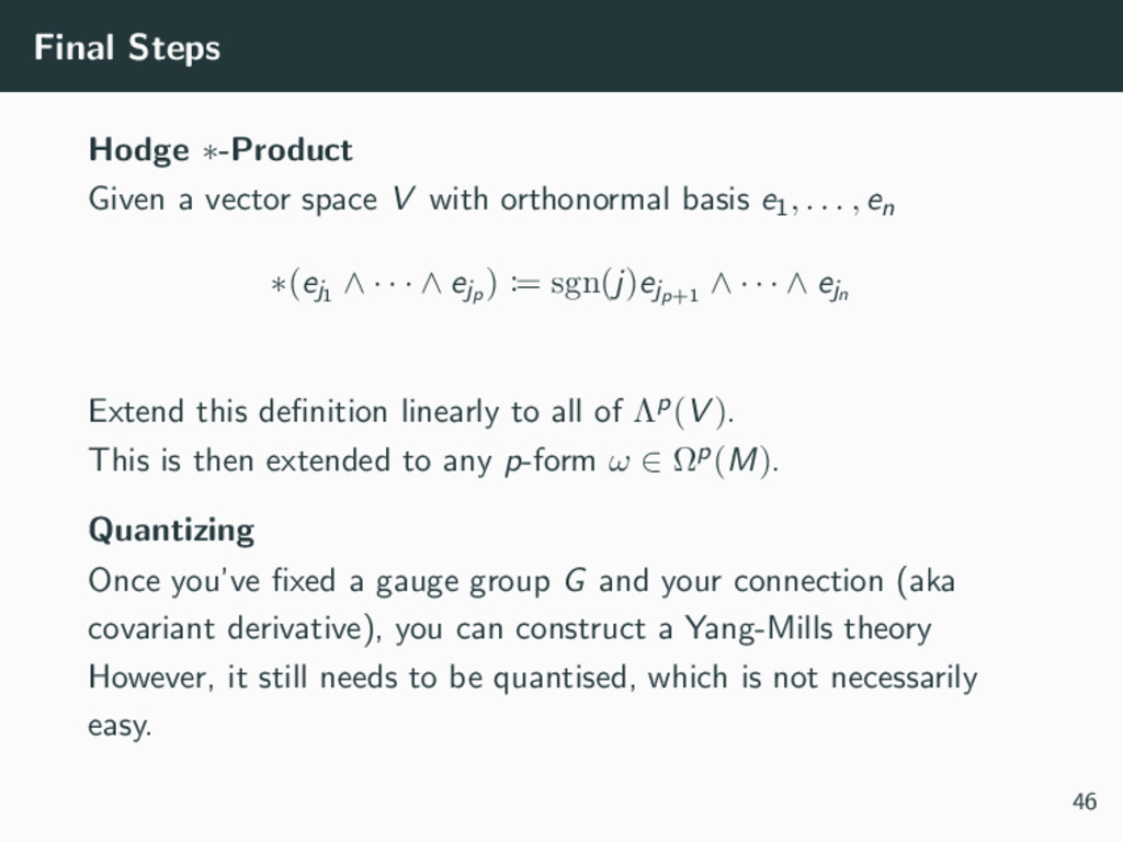
orthonormal basis e1, . . . , en ∗(ej1 ∧ · · · ∧ ejp ) := sgn(j)ejp+1 ∧ · · · ∧ ejn Extend this definition linearly to all of Λp(V ). This is then extended to any p-form ω ∈ Ωp(M). Quantizing Once you’ve fixed a gauge group G and your connection (aka covariant derivative), you can construct a Yang-Mills theory However, it still needs to be quantised, which is not necessarily easy. 46
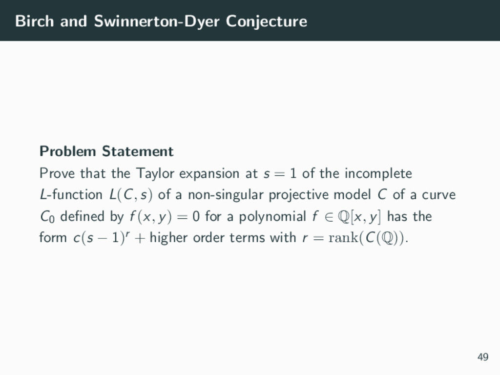
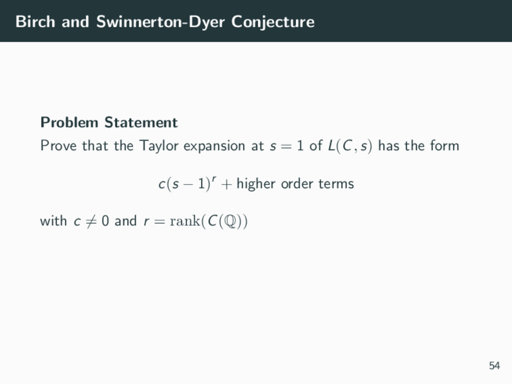
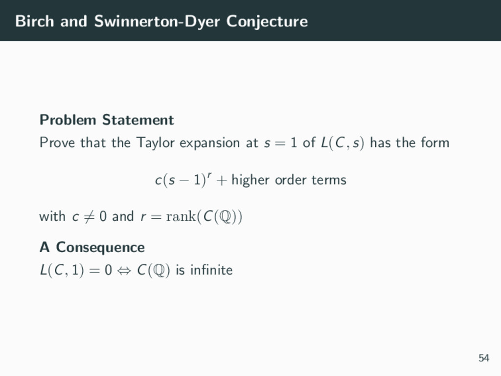
expansion at s = 1 of the incomplete L-function L(C, s) of a non-singular projective model C of a curve C0 defined by f (x, y) = 0 for a polynomial f ∈ Q[x, y] has the form c(s − 1)r + higher order terms with r = rank(C(Q)). 49
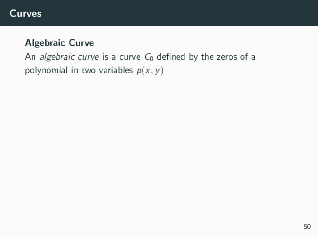
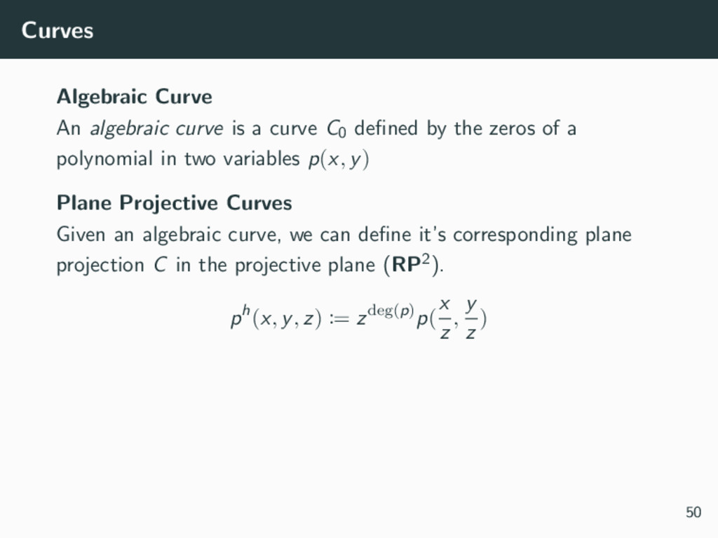
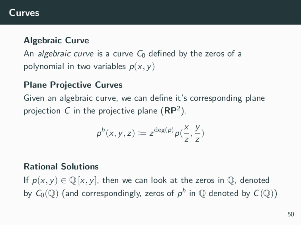
defined by the zeros of a polynomial in two variables p(x, y) Plane Projective Curves Given an algebraic curve, we can define it’s corresponding plane projection C in the projective plane (RP2). ph(x, y, z) := zdeg(p)p( x z , y z ) 50
defined by the zeros of a polynomial in two variables p(x, y) Plane Projective Curves Given an algebraic curve, we can define it’s corresponding plane projection C in the projective plane (RP2). ph(x, y, z) := zdeg(p)p( x z , y z ) Rational Solutions If p(x, y) ∈ Q [x, y], then we can look at the zeros in Q, denoted by C0(Q) (and correspondingly, zeros of ph in Q denoted by C(Q)) 50
finite, or they are both infinite Genus of Curves Plane projective curves C can be characterized by their genus , and we call the genus of C the genus of C0 too 51
finite, or they are both infinite Genus of Curves Plane projective curves C can be characterized by their genus , and we call the genus of C the genus of C0 too There are results about the size of C0(Q) for genus ≥ 2 and 0, but genus 1 remains open in general 51
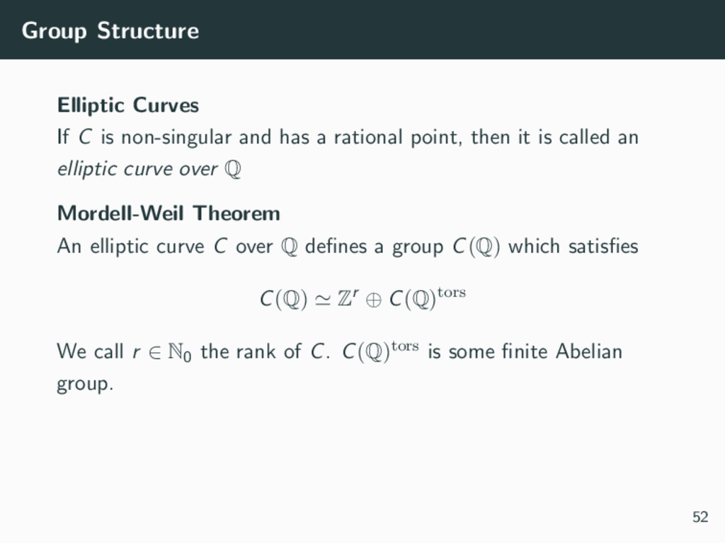
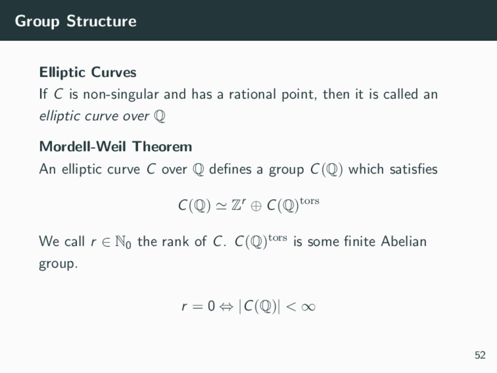
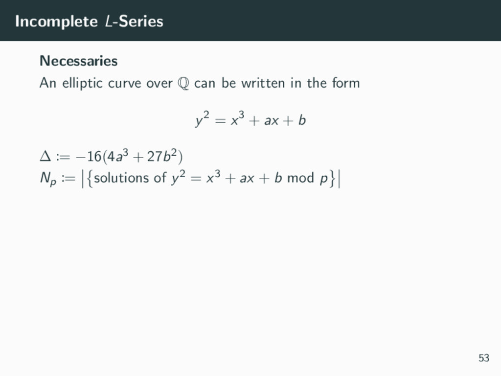
a rational point, then it is called an elliptic curve over Q Mordell-Weil Theorem An elliptic curve C over Q defines a group C(Q) which satisfies C(Q) Zr ⊕ C(Q)tors 52
a rational point, then it is called an elliptic curve over Q Mordell-Weil Theorem An elliptic curve C over Q defines a group C(Q) which satisfies C(Q) Zr ⊕ C(Q)tors We call r ∈ N0 the rank of C. C(Q)tors is some finite Abelian group. 52
a rational point, then it is called an elliptic curve over Q Mordell-Weil Theorem An elliptic curve C over Q defines a group C(Q) which satisfies C(Q) Zr ⊕ C(Q)tors We call r ∈ N0 the rank of C. C(Q)tors is some finite Abelian group. r = 0 ⇔ |C(Q)| < ∞ 52
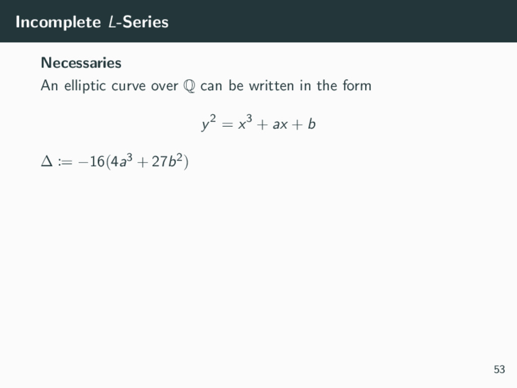
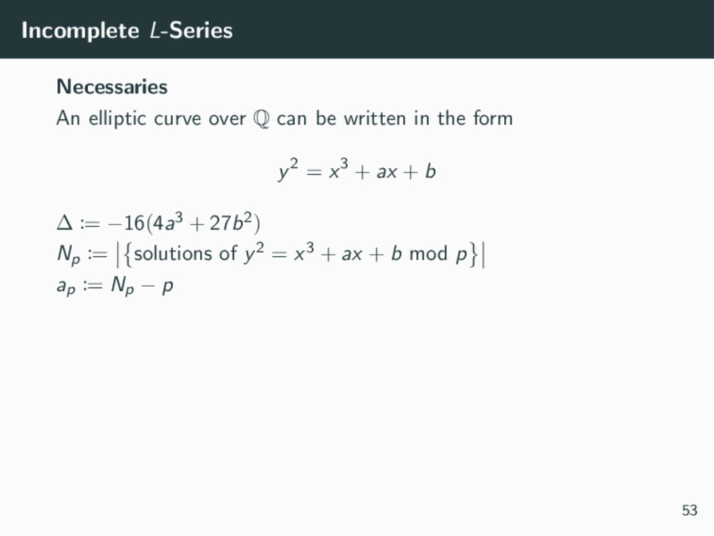
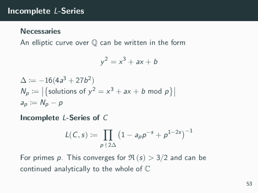
written in the form y2 = x3 + ax + b ∆ := −16(4a3 + 27b2) Np := solutions of y2 = x3 + ax + b mod p ap := Np − p Incomplete L-Series of C L(C, s) := p 2∆ 1 − app−s + p1−2s −1 For primes p. This converges for R (s) > 3/2 and can be continued analytically to the whole of C 53