models Geometric flow for biomolecular solvation Jaehun Chun1, Dennis Thomas1, Michael Daily1, Luke Gosink1, Emilie Hogan1, Zhan Chen2, Guowei Wei2, Nathan Baker1 1Pacific Northwest National Laboratory 2Department of Mathematics Michigan State University May-2013 Baker et al Geometric flow (PNWD-SA-10081)
models Acknowledgments Team members Jaehun Chun Luke Gosink Tyler Harmon Emilie Hogan Andrew Stevens Dennis Thomas Guowei Wei Collaborators Jens E. Nielsen pKa co-op Bertrand Garcia-Moreno Marilyn Gunner Julie Mitchell Mike Holst Funding NIH R01 GM069702 NIH R01 GM090208 NIH National Biomedical Computation Resource Baker et al Geometric flow (PNWD-SA-10081)
models Research topics Nanotechnology research Outline Research overview Research topics Nanotechnology research Background on biomolecular solvation Relevance and objectives Continuum solvation models Scalable numerical methods Caveats in current approaches New self-consistent continuum solvation models Model description Numerical approach Applications Next steps Baker et al Geometric flow (PNWD-SA-10081)
models Research topics Nanotechnology research Research overview Solvation modeling Theory Computational methods Nanomaterial modeling Informatics Structure-activity relationships Simulation Biological membrane modeling Signature discovery (http://signatures.pnnl.gov) Baker et al Geometric flow (PNWD-SA-10081)
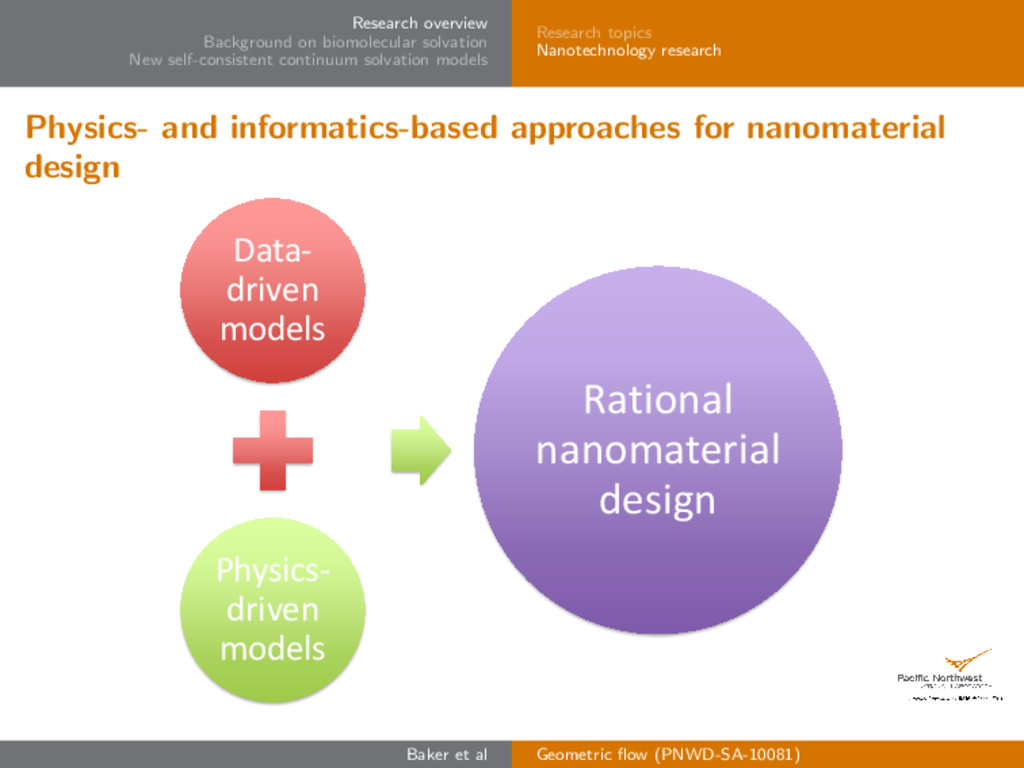
models Research topics Nanotechnology research Physics- and informatics-based approaches for nanomaterial design Data- driven models Physics- driven models Rational nanomaterial design Baker et al Geometric flow (PNWD-SA-10081)
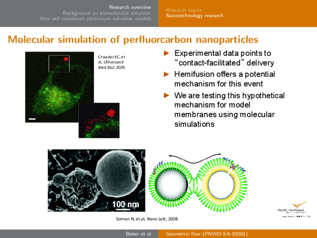
models Research topics Nanotechnology research Molecular simulation of perfluorcarbon nanoparticles Experimental data points to “contact-facilitated” delivery Hemifusion offers a potential mechanism for this event We are testing this hypothetical mechanism for model membranes using molecular simulations Crowder KC, et al, Ultrasound Med Biol, 2005 Soman N, et al, Nano Lett, 2008. Baker et al Geometric flow (PNWD-SA-10081)
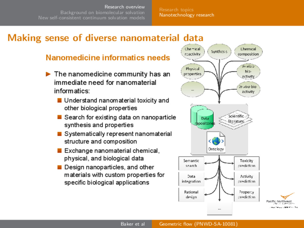
models Research topics Nanotechnology research Making sense of diverse nanomaterial data Nanomedicine informatics needs The nanomedicine community has an immediate need for nanomaterial informatics: Understand nanomaterial toxicity and other biological properties Search for existing data on nanoparticle synthesis and properties Systematically represent nanomaterial structure and composition Exchange nanomaterial chemical, physical, and biological data Design nanoparticles, and other materials with custom properties for specific biological applications Baker et al Geometric flow (PNWD-SA-10081)
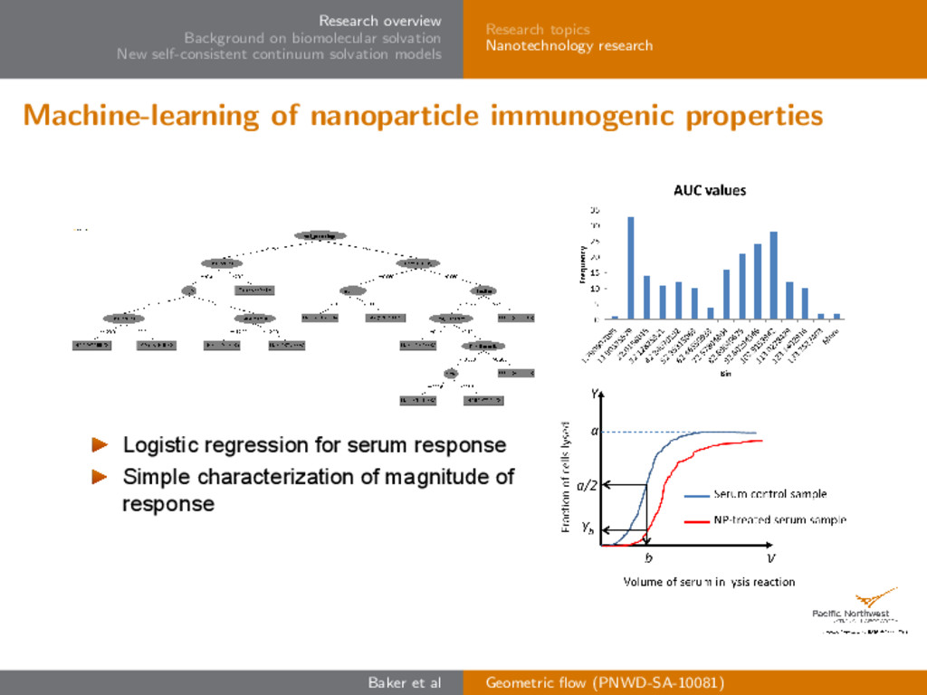
models Research topics Nanotechnology research Machine-learning of nanoparticle immunogenic properties Logistic regression for serum response Simple characterization of magnitude of response Baker et al Geometric flow (PNWD-SA-10081)
models Relevance and objectives Continuum solvation models Scalable numerical methods Caveats in current approaches Outline Research overview Research topics Nanotechnology research Background on biomolecular solvation Relevance and objectives Continuum solvation models Scalable numerical methods Caveats in current approaches New self-consistent continuum solvation models Model description Numerical approach Applications Next steps Baker et al Geometric flow (PNWD-SA-10081)
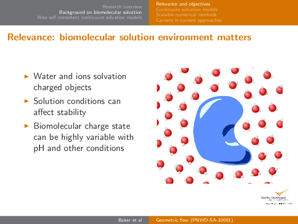
models Relevance and objectives Continuum solvation models Scalable numerical methods Caveats in current approaches Relevance: biomolecular solution environment matters Water and ions solvation charged objects Solution conditions can affect stability Biomolecular charge state can be highly variable with pH and other conditions Baker et al Geometric flow (PNWD-SA-10081)
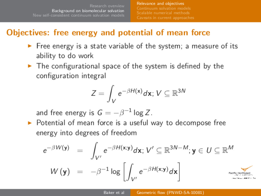
models Relevance and objectives Continuum solvation models Scalable numerical methods Caveats in current approaches Objectives: free energy and potential of mean force Free energy is a state variable of the system; a measure of its ability to do work The configurational space of the system is defined by the configuration integral Z = V e−βH(x)dx; V ⊆ R3N and free energy is G = −β−1 log Z. Potential of mean force is a useful way to decompose free energy into degrees of freedom e−βW (y) = V e−βH(x;y)dx; V ⊆ R3N−M; y ∈ U ⊆ RM W (y) = −β−1 log V e−βH(x;y)dx Baker et al Geometric flow (PNWD-SA-10081)
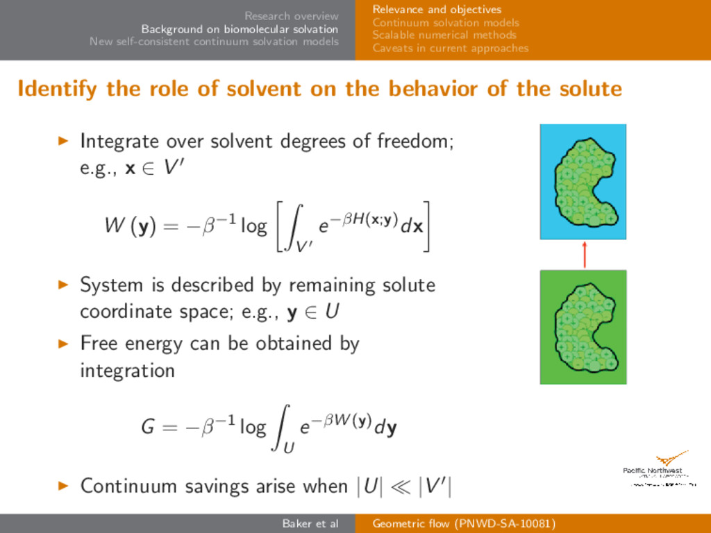
models Relevance and objectives Continuum solvation models Scalable numerical methods Caveats in current approaches Identify the role of solvent on the behavior of the solute Integrate over solvent degrees of freedom; e.g., x ∈ V W (y) = −β−1 log V e−βH(x;y)dx System is described by remaining solute coordinate space; e.g., y ∈ U Free energy can be obtained by integration G = −β−1 log U e−βW (y)dy Continuum savings arise when |U| |V | Baker et al Geometric flow (PNWD-SA-10081)
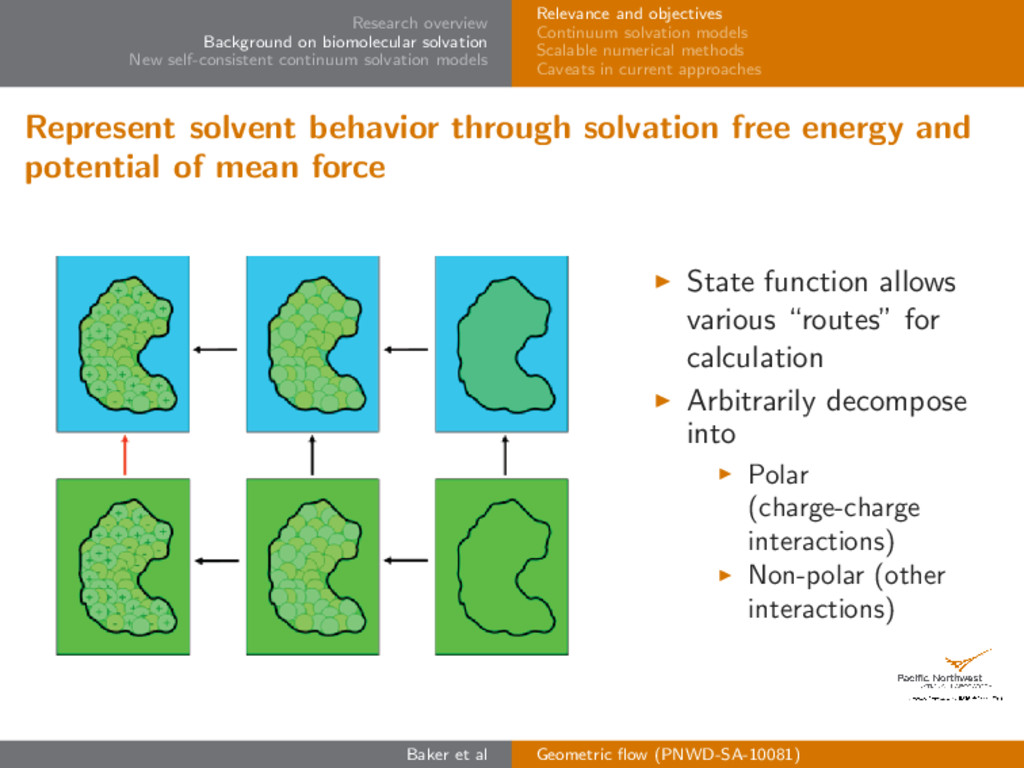
models Relevance and objectives Continuum solvation models Scalable numerical methods Caveats in current approaches Represent solvent behavior through solvation free energy and potential of mean force State function allows various “routes” for calculation Arbitrarily decompose into Polar (charge-charge interactions) Non-polar (other interactions) Baker et al Geometric flow (PNWD-SA-10081)
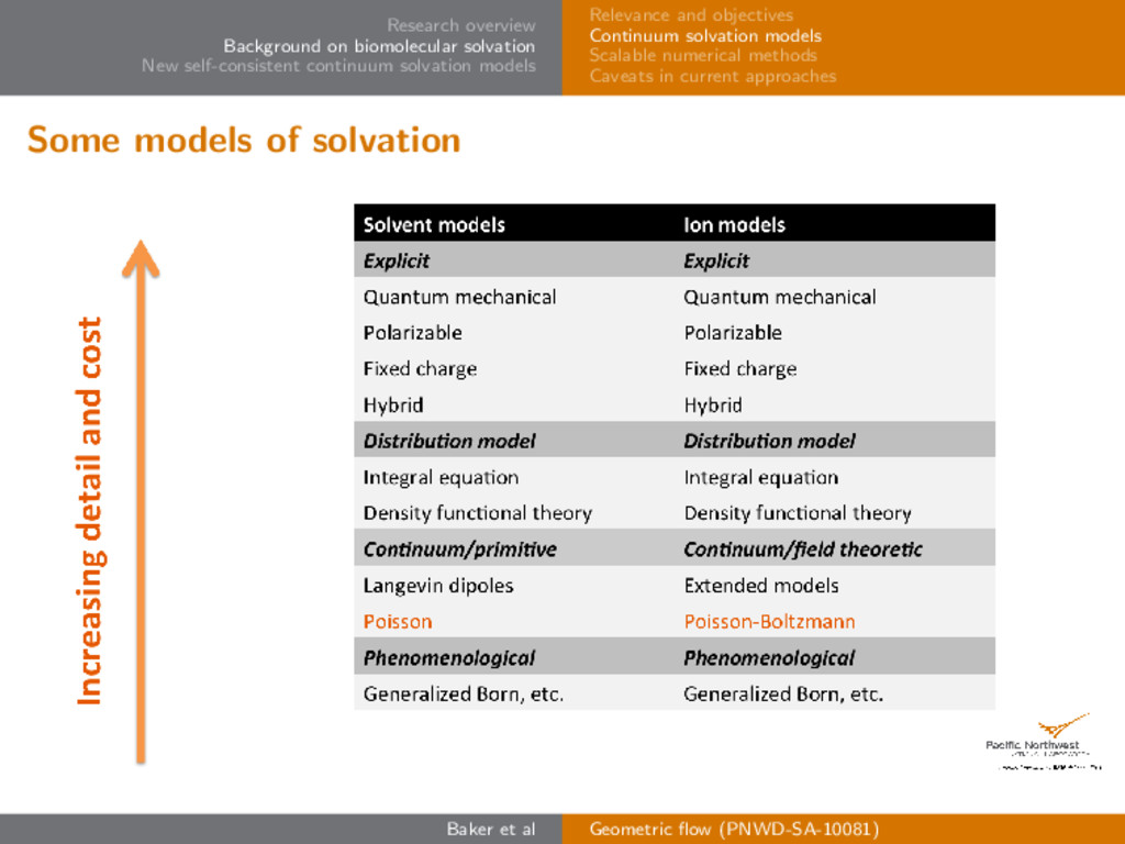
models Relevance and objectives Continuum solvation models Scalable numerical methods Caveats in current approaches Some models of solvation Baker et al Geometric flow (PNWD-SA-10081)
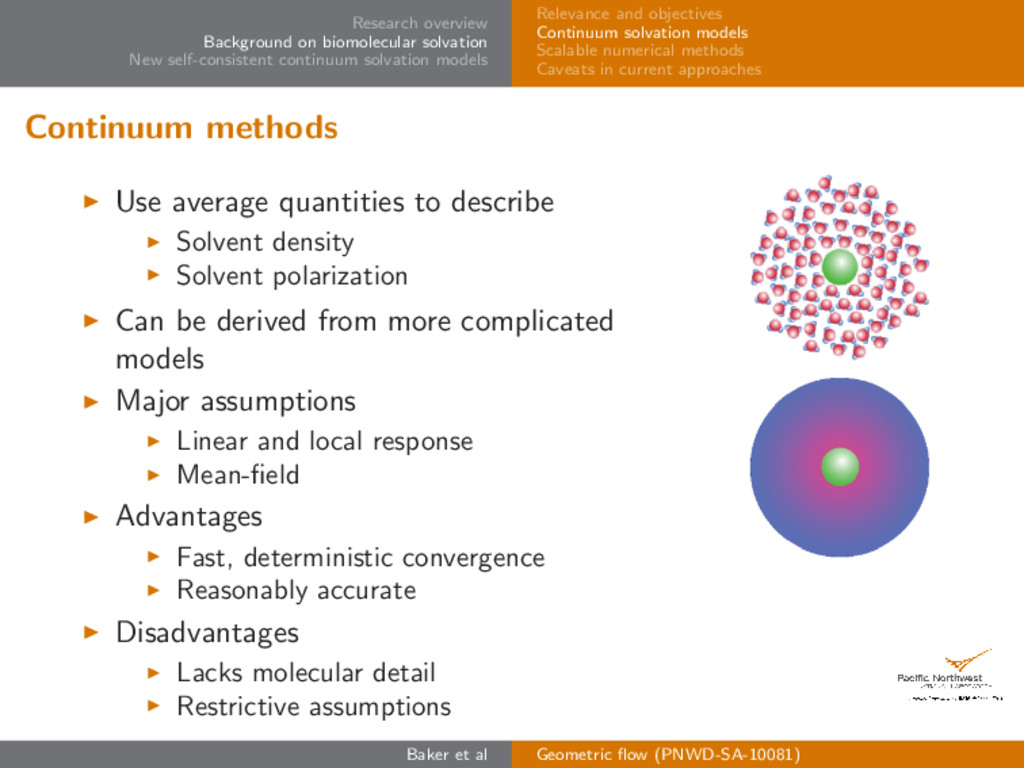
models Relevance and objectives Continuum solvation models Scalable numerical methods Caveats in current approaches Continuum methods Use average quantities to describe Solvent density Solvent polarization Can be derived from more complicated models Major assumptions Linear and local response Mean-field Advantages Fast, deterministic convergence Reasonably accurate Disadvantages Lacks molecular detail Restrictive assumptions Baker et al Geometric flow (PNWD-SA-10081)
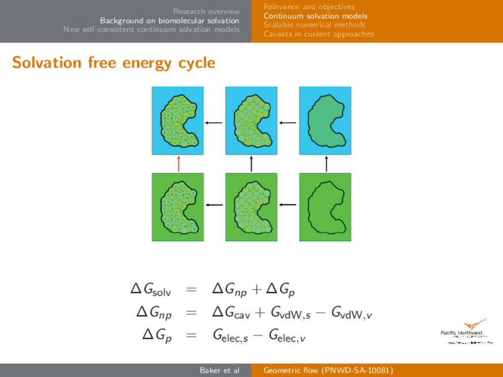
models Relevance and objectives Continuum solvation models Scalable numerical methods Caveats in current approaches Continuum description of solvation free energy Solvation free energy artificially decomposed into polar and nonpolar components: ∆G = ∆Gnp + ∆Gp Nonpolar term described by energy of inserting uncharged solute into solution Polar term described by energy of inserting charged solute into solution Baker et al Geometric flow (PNWD-SA-10081)
models Relevance and objectives Continuum solvation models Scalable numerical methods Caveats in current approaches Nonpolar solvation free energy Modeled by a perturbation from creation of a hard-wall potential cavity in Lennard-Jones solvent ∆Gnp = ∆Gcav + GvdW,s − GvdW,v All energies defined in terms of solvent density χ(x) Approximate cavity energy using scaled particle theory ∆Gcav ≈ G0[χ] + pV [χ] + γA[χ] + . . . Approximate perturbation by convolution of solvent density with dispersive Lennard-Jones interaction with solute GvdW,s − GvdW,v ≈ ρ Na i χ(x)uvdW(x − xi )dx Baker et al Geometric flow (PNWD-SA-10081)
models Relevance and objectives Continuum solvation models Scalable numerical methods Caveats in current approaches Polar solvation energy Modeled by Poisson-Boltzmann theory GPB,s = Gpol + Gq + Gion Continuum solvent assumptions Linear and local dielectric response: functional of solvent density χ and electrostatic potential φ Gpol + Gq ≈ Ω − 1 2 (∇φ)2 + φ dx Could subtract vacuum-state energy for “regularized” form Mean-field ionic response: functional of electrostatic potential φ; dependent on ion-solute interaction potential V (χ) Gion ≈ −β−1 Ω ci e−βVi e−βqi φ − 1 dx Baker et al Geometric flow (PNWD-SA-10081)
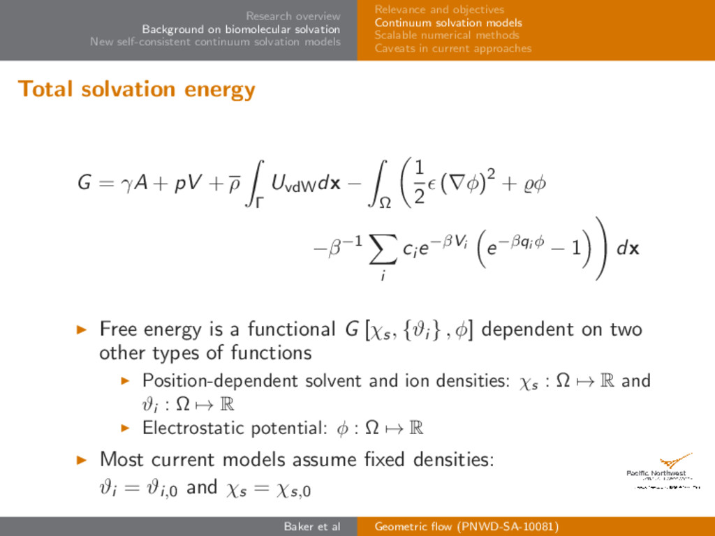
models Relevance and objectives Continuum solvation models Scalable numerical methods Caveats in current approaches Total solvation energy G = γA + pV + ρ Γ UvdWdx − Ω 1 2 (∇φ)2 + φ −β−1 i ci e−βVi e−βqi φ − 1 dx Free energy is a functional G [χs, {ϑi } , φ] dependent on two other types of functions Position-dependent solvent and ion densities: χs : Ω → R and ϑi : Ω → R Electrostatic potential: φ : Ω → R Most current models assume fixed densities: ϑi = ϑi,0 and χs = χs,0 Baker et al Geometric flow (PNWD-SA-10081)
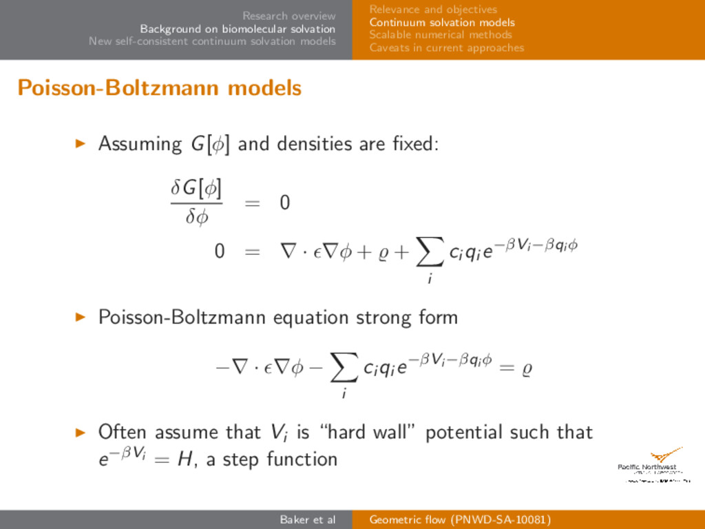
models Relevance and objectives Continuum solvation models Scalable numerical methods Caveats in current approaches Poisson-Boltzmann models Assuming G[φ] and densities are fixed: δG[φ] δφ = 0 0 = ∇ · ∇φ + + i ci qi e−βVi −βqi φ Poisson-Boltzmann equation strong form −∇ · ∇φ − i ci qi e−βVi −βqi φ = Often assume that Vi is “hard wall” potential such that e−βVi = H, a step function Baker et al Geometric flow (PNWD-SA-10081)
models Relevance and objectives Continuum solvation models Scalable numerical methods Caveats in current approaches Poisson-Boltzmann equation Baker et al Geometric flow (PNWD-SA-10081)
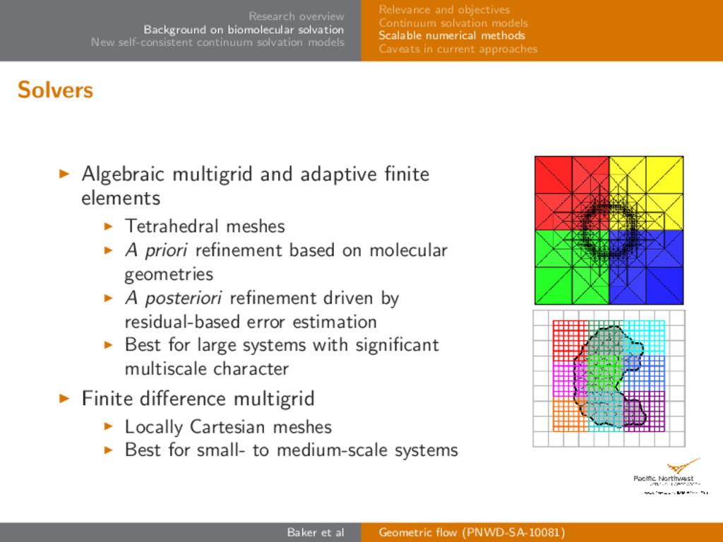
models Relevance and objectives Continuum solvation models Scalable numerical methods Caveats in current approaches Solvers Algebraic multigrid and adaptive finite elements Tetrahedral meshes A priori refinement based on molecular geometries A posteriori refinement driven by residual-based error estimation Best for large systems with significant multiscale character Finite difference multigrid Locally Cartesian meshes Best for small- to medium-scale systems Baker et al Geometric flow (PNWD-SA-10081)
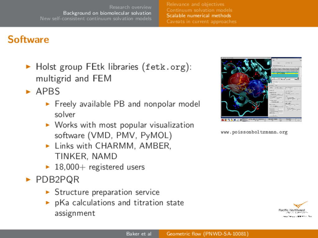
models Relevance and objectives Continuum solvation models Scalable numerical methods Caveats in current approaches Software Holst group FEtk libraries (fetk.org): multigrid and FEM APBS Freely available PB and nonpolar model solver Works with most popular visualization software (VMD, PMV, PyMOL) Links with CHARMM, AMBER, TINKER, NAMD 18,000+ registered users PDB2PQR Structure preparation service pKa calculations and titration state assignment www.poissonboltzmann.org Baker et al Geometric flow (PNWD-SA-10081)
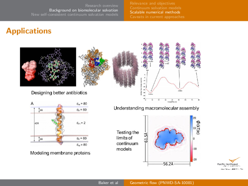
models Relevance and objectives Continuum solvation models Scalable numerical methods Caveats in current approaches Applications Baker et al Geometric flow (PNWD-SA-10081)
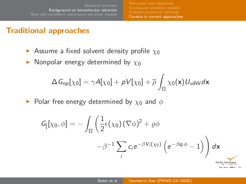
models Relevance and objectives Continuum solvation models Scalable numerical methods Caveats in current approaches Traditional approaches Assume a fixed solvent density profile χ0 Nonpolar energy determined by χ0 ∆Gnp[χ0] = γA[χ0] + pV [χ0] + ρ Ω χ0(x)UvdWdx Polar free energy determined by χ0 and φ G[ [χ0, φ] = − Ω 1 2 (χ0) (∇φ)2 + φ −β−1 i ci e−βVi (χ0) e−βqi φ − 1 dx Baker et al Geometric flow (PNWD-SA-10081)
models Relevance and objectives Continuum solvation models Scalable numerical methods Caveats in current approaches Caveats Arbitrary surface definitions for , e−βVi , A, and V Difficult to relate force field radii to coefficient definitions Different parameters often needed for polar and apolar solvation Inability to couple polar and nonpolar interactions Unable to describe strong density changes near polar/nonpolar interfaces Different models for polar and nonpolar interactions Baker et al Geometric flow (PNWD-SA-10081)
models Model description Numerical approach Applications Next steps Outline Research overview Research topics Nanotechnology research Background on biomolecular solvation Relevance and objectives Continuum solvation models Scalable numerical methods Caveats in current approaches New self-consistent continuum solvation models Model description Numerical approach Applications Next steps Baker et al Geometric flow (PNWD-SA-10081)
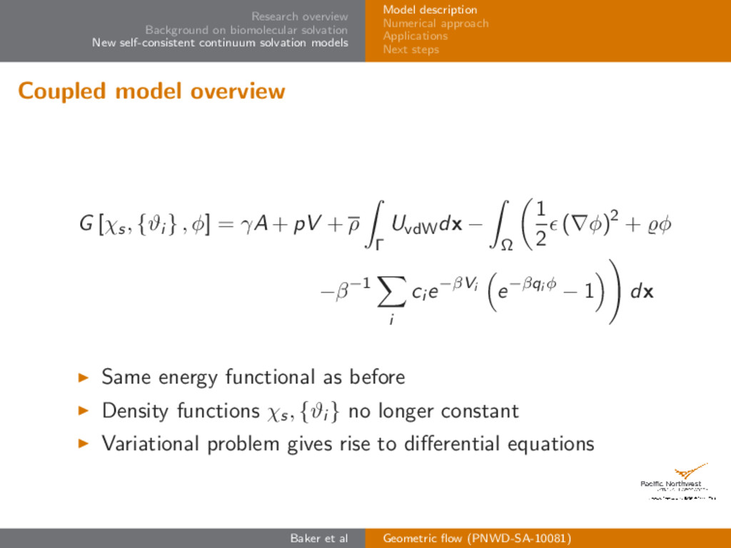
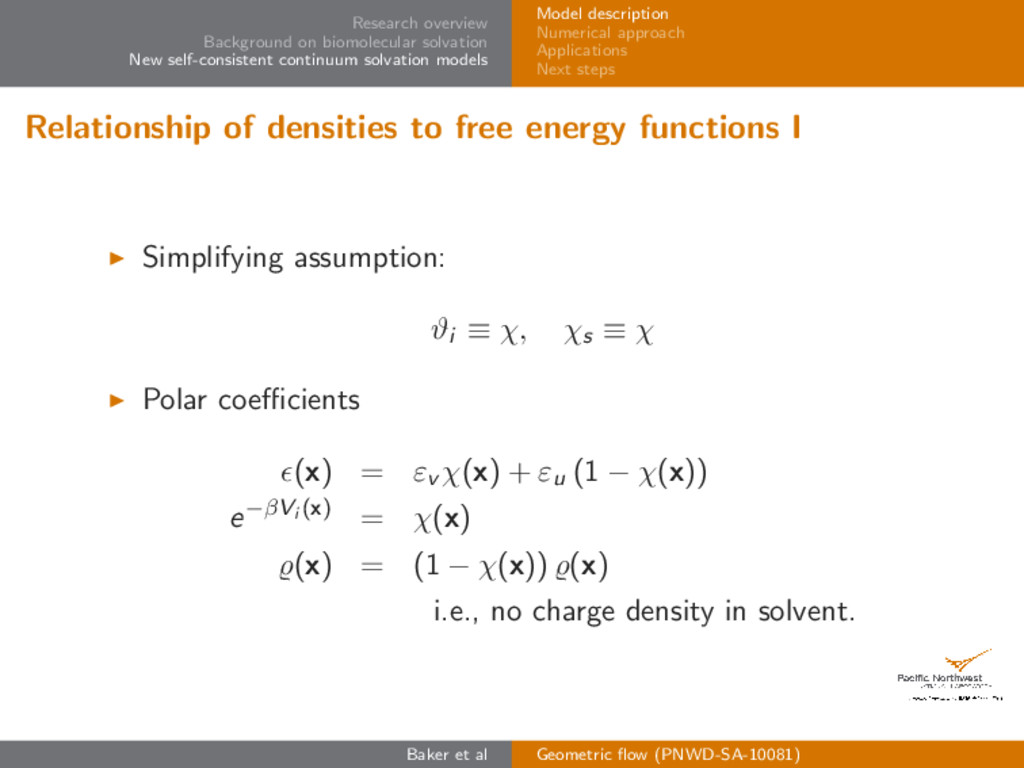
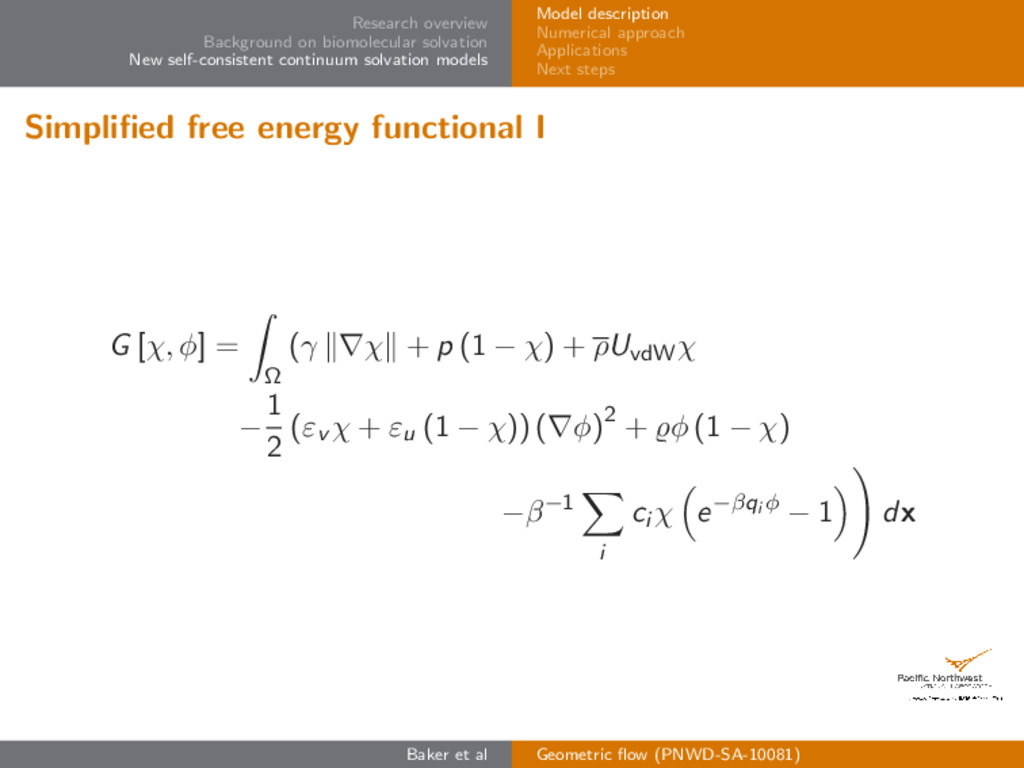
models Model description Numerical approach Applications Next steps Coupled model overview G [χs, {ϑi } , φ] = γA + pV + ρ Γ UvdWdx − Ω 1 2 (∇φ)2 + φ −β−1 i ci e−βVi e−βqi φ − 1 dx Same energy functional as before Density functions χs, {ϑi } no longer constant Variational problem gives rise to differential equations Baker et al Geometric flow (PNWD-SA-10081)
models Model description Numerical approach Applications Next steps Relationship of densities to free energy functions II Nonpolar coefficients (using coarea formula) V = Ω (1 − χ(x)) dx A = Ω ∇χ(x) dx Γ UvdW(x)dx = Ω UvdW(x)χ(x)dx Baker et al Geometric flow (PNWD-SA-10081)
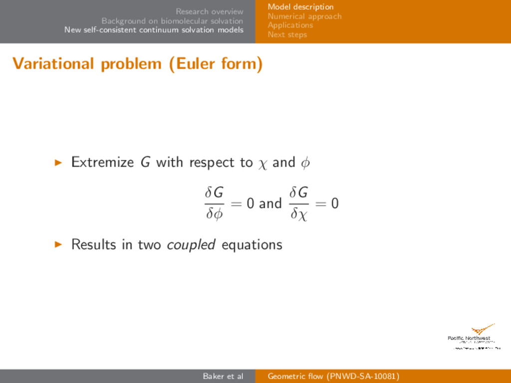
models Model description Numerical approach Applications Next steps Variational problem (Euler form) Extremize G with respect to χ and φ δG δφ = 0 and δG δχ = 0 Results in two coupled equations Baker et al Geometric flow (PNWD-SA-10081)
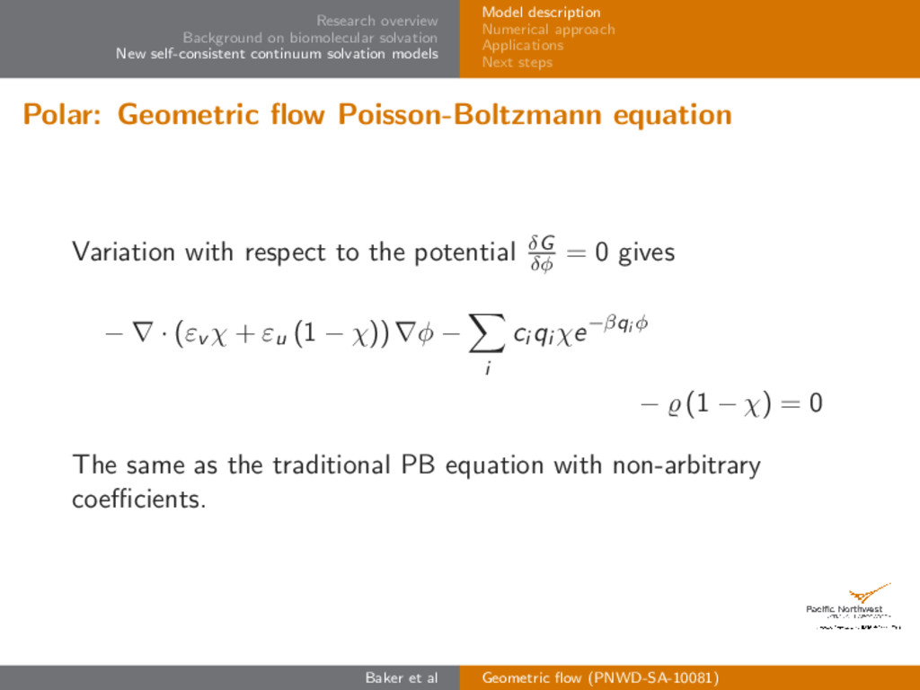
models Model description Numerical approach Applications Next steps Polar: Geometric flow Poisson-Boltzmann equation Variation with respect to the potential δG δφ = 0 gives − ∇ · (εv χ + εu (1 − χ)) ∇φ − i ci qi χe−βqi φ − (1 − χ) = 0 The same as the traditional PB equation with non-arbitrary coefficients. Baker et al Geometric flow (PNWD-SA-10081)
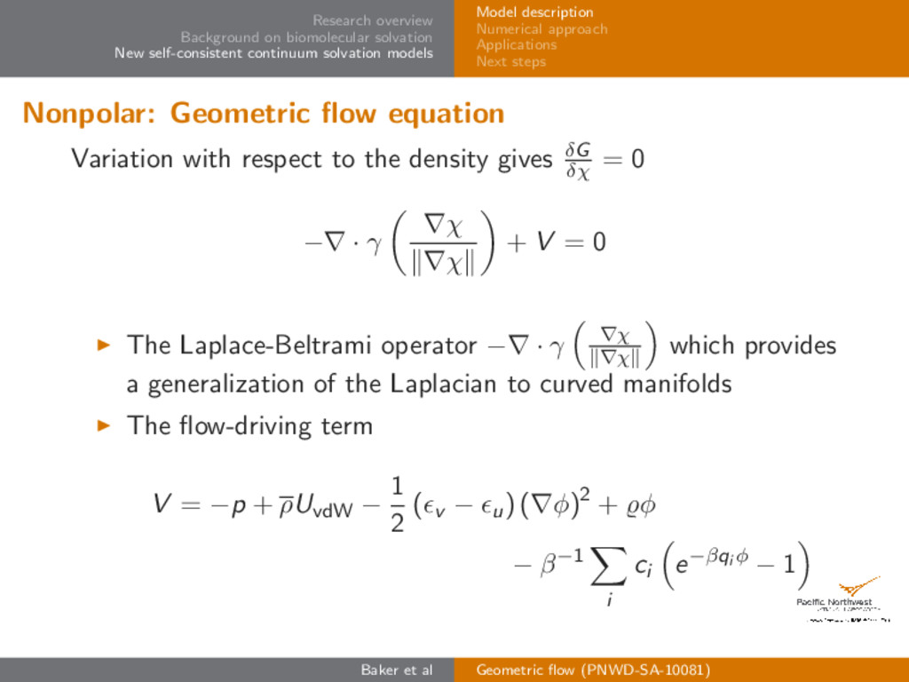
models Model description Numerical approach Applications Next steps Nonpolar: Geometric flow equation Variation with respect to the density gives δG δχ = 0 −∇ · γ ∇χ ∇χ + V = 0 The Laplace-Beltrami operator −∇ · γ ∇χ ∇χ which provides a generalization of the Laplacian to curved manifolds The flow-driving term V = −p + ρUvdW − 1 2 ( v − u) (∇φ)2 + φ − β−1 i ci e−βqi φ − 1 Baker et al Geometric flow (PNWD-SA-10081)
models Model description Numerical approach Applications Next steps The coupled system expressed as a parabolic problem Geometric flow ∂χ ∂t = ∇χ ∇ · γ ∇χ ∇χ + ˜ V Time-stepping Euler or ADI scheme Iterative solution of geometric flow and linearized Poisson-Boltzmann equations Relaxation for ˜ V updates Baker et al Geometric flow (PNWD-SA-10081)
models Model description Numerical approach Applications Next steps Discretization and solvers Current: Finite difference discretization Bi-conjugate gradient solver Incomplete LU preconditioning Future: Wei group Matched Interface Boundary method Parallel multigrid for low-frequency features Adaptive multilevel finite elements Initial conditions use “inflated” surface Convergence measured by energy, volume, area Baker et al Geometric flow (PNWD-SA-10081)
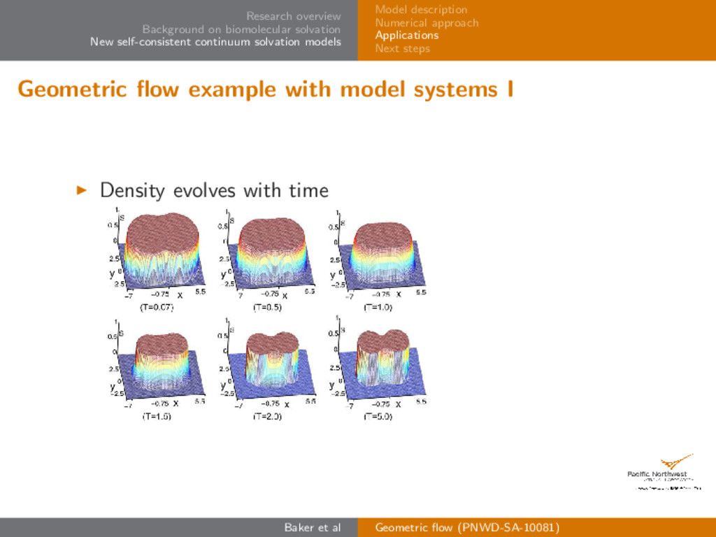
models Model description Numerical approach Applications Next steps Geometric flow example with model systems I Density evolves with time Baker et al Geometric flow (PNWD-SA-10081)
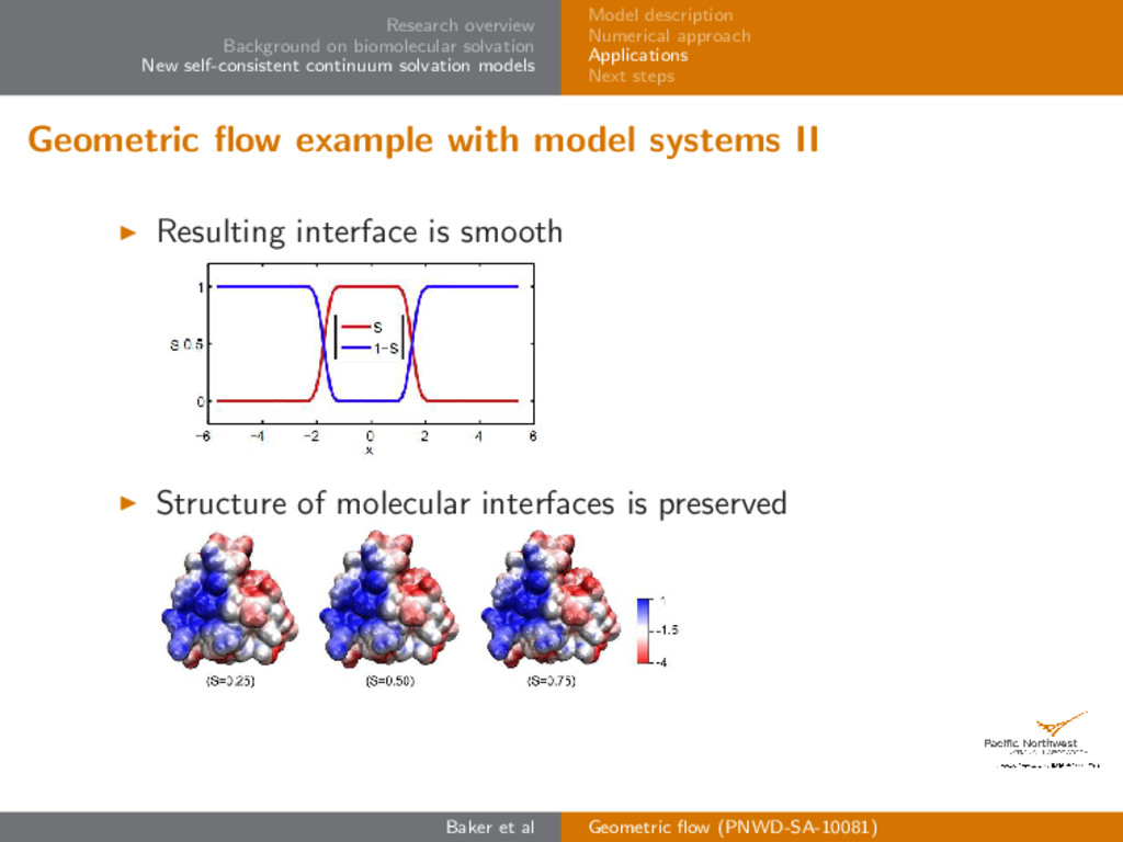
models Model description Numerical approach Applications Next steps Geometric flow example with model systems II Resulting interface is smooth Structure of molecular interfaces is preserved Baker et al Geometric flow (PNWD-SA-10081)
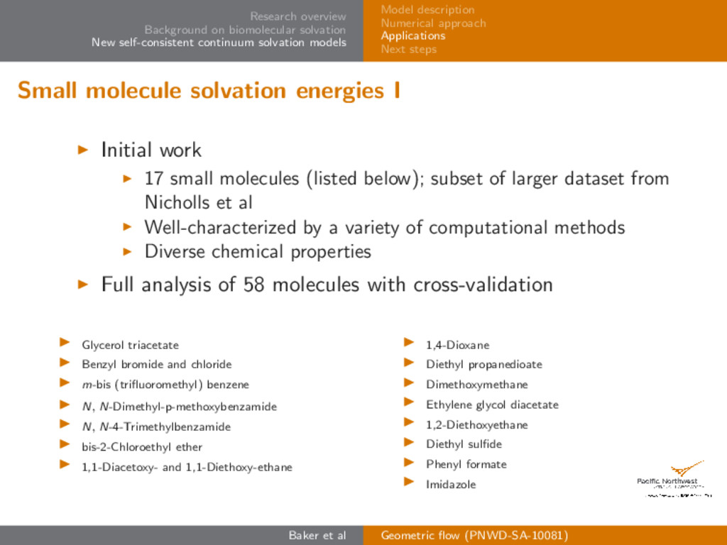
models Model description Numerical approach Applications Next steps Small molecule solvation energies I Initial work 17 small molecules (listed below); subset of larger dataset from Nicholls et al Well-characterized by a variety of computational methods Diverse chemical properties Full analysis of 58 molecules with cross-validation Glycerol triacetate Benzyl bromide and chloride m-bis (trifluoromethyl) benzene N, N-Dimethyl-p-methoxybenzamide N, N-4-Trimethylbenzamide bis-2-Chloroethyl ether 1,1-Diacetoxy- and 1,1-Diethoxy-ethane 1,4-Dioxane Diethyl propanedioate Dimethoxymethane Ethylene glycol diacetate 1,2-Diethoxyethane Diethyl sulfide Phenyl formate Imidazole Baker et al Geometric flow (PNWD-SA-10081)
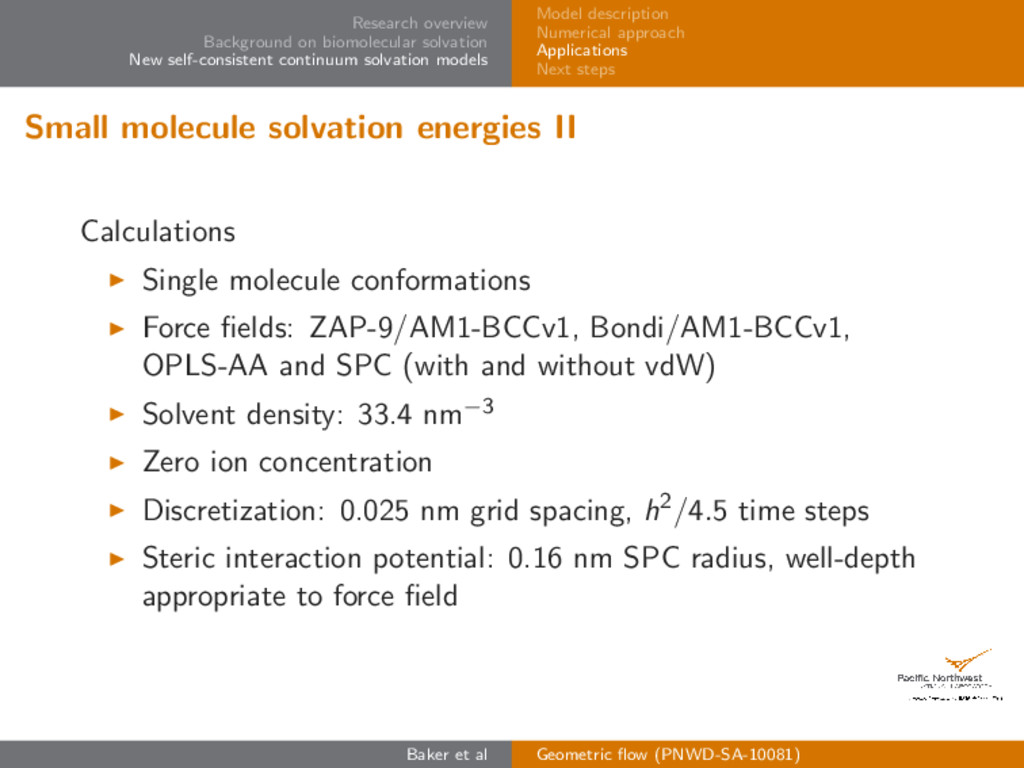
models Model description Numerical approach Applications Next steps Small molecule solvation energies II Calculations Single molecule conformations Force fields: ZAP-9/AM1-BCCv1, Bondi/AM1-BCCv1, OPLS-AA and SPC (with and without vdW) Solvent density: 33.4 nm−3 Zero ion concentration Discretization: 0.025 nm grid spacing, h2/4.5 time steps Steric interaction potential: 0.16 nm SPC radius, well-depth appropriate to force field Baker et al Geometric flow (PNWD-SA-10081)
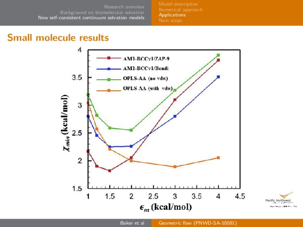
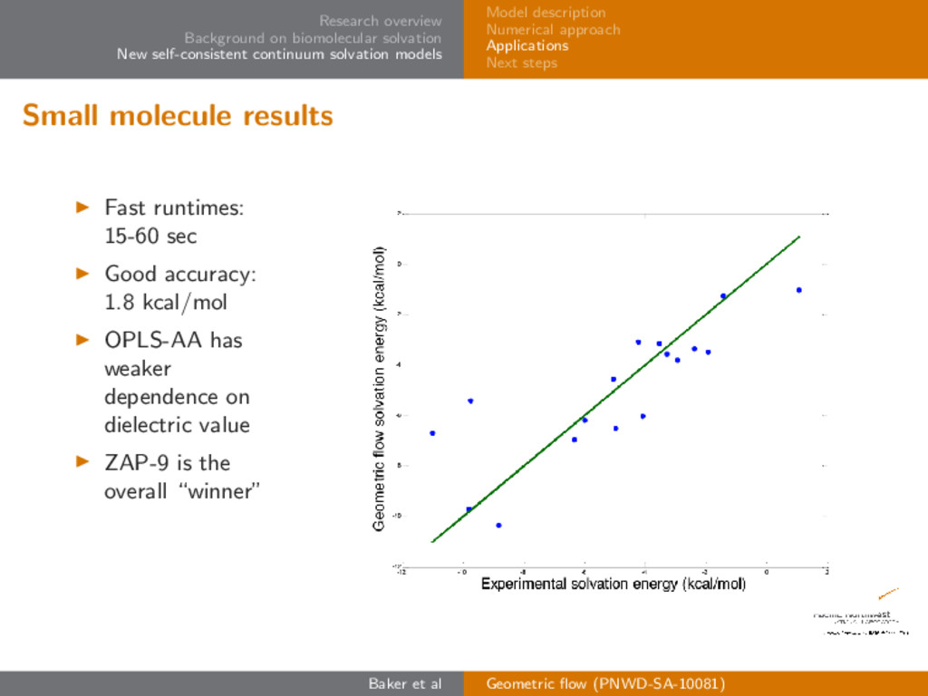
models Model description Numerical approach Applications Next steps Small molecule results Fast runtimes: 15-60 sec Good accuracy: 1.8 kcal/mol OPLS-AA has weaker dependence on dielectric value ZAP-9 is the overall “winner” Baker et al Geometric flow (PNWD-SA-10081)
models Model description Numerical approach Applications Next steps Conclusions and next steps Benefits of this model Self-consistent treatment of polar and nonpolar energetics Very few adjustable parameters: Solvent density Dielectric values Solute and solvent force field Good accuracy for small molecules Next steps Resolve physical origins of parameter degeneracy Solver speed improvement Model improvement Application to molecular binding energies and pKas Integration with other continuum models (mechanics, hydrodynamics, etc.) Baker et al Geometric flow (PNWD-SA-10081)
models Model description Numerical approach Applications Next steps Acknowledgments Team members Jaehun Chun Luke Gosink Tyler Harmon Emilie Hogan Andrew Stevens Dennis Thomas Guowei Wei Collaborators Jens E. Nielsen pKa co-op Bertrand Garcia-Moreno Marilyn Gunner Julie Mitchell Mike Holst Funding NIH R01 GM069702 NIH R01 GM090208 NIH National Biomedical Computation Resource Baker et al Geometric flow (PNWD-SA-10081)