NoSql Paper

NoSql Databases

Abstract In today’s time, data is everything. With services like
Gmail, Facebook, Google+ and others getting more popular, its getting difficult to manage huge amounts of data, its availability, consistency and throughput because of which a new breed of databases called as NoSql databases have come into picture. I aim to study the three different NoSql databases, Amazon DynamoDB, Riak DB, MongoDB and then see how well do they solve the problem faced by some of the biggest companies in the world.

Table of Contents Chapter 1 ................................................................................................................................................................. 8 Introduction ............................................................................................................................................................................
8 Why NoSql? ............................................................................................................................................................................. 8 What does NoSql Database enable us with? .............................................................................................................. 2 CAP Theorem ( Brewer’s Theorem ) ............................................................................................................................ 3 Different Types of NoSql databases .............................................................................................................................. 4 Key-‐/Value-‐Stores ................................................................................................................................................................ 4 Document Databases ........................................................................................................................................................... 4 Chapter 2 ................................................................................................................................................................. 5 Amazon’s DynamoDB .......................................................................................................................................................... 5 Context and Requirements at Amazon ........................................................................................................................ 5 Design considerations ......................................................................................................................................................... 6 Partitioning Algorithm ....................................................................................................................................................... 9 Replication ............................................................................................................................................................................... 9 Chapter 3 .............................................................................................................................................................. 10 Riak DB ................................................................................................................................................................................... 10 Riak Core Concepts ........................................................................................................................................................... 11 Read an Object ................................................................................................................... 12 Adding an Object ................................................................................................................ 12 Updating an Object ............................................................................................................. 13 Deleting an Object .............................................................................................................. 14 Map Reduce .......................................................................................................................................................................... 14 When should you use map reduce? ........................................................................................................... 14 How it works ........................................................................................................................ 15 Chapter 4 .............................................................................................................................................................. 17 MongoDB ............................................................................................................................................................................... 17 Overview ............................................................................................................................. 17 Collections .......................................................................................................................... 17 Documents .......................................................................................................................... 18 Data types for attributes within a document .............................................................................................. 19 Relationship between documents ....................................................................................... 20 Database Operations .............................................................................................................................................. 21 Queries .................................................................................................................................................................... 21 Cursors ................................................................................................................................................................... 22 Query Optimizers ................................................................................................................ 22 Atomic Updates ................................................................................................................................................... 23 Removing Data .................................................................................................................................................... 23 Aggregation .......................................................................................................................................................... 24 Returning the Number of Documents with Count () .......................................................................... 24 Retrieving Unique Values with Distinct() ............................................................................................... 24 Grouping your results ...................................................................................................................................... 25 Map Reduce ........................................................................................................................ 25 Indexes ............................................................................................................................... 27 Geo-‐spatial Indexing ......................................................................................................................................... 28

Profiling Queries ................................................................................................................. 28 Distribution Aspects ............................................................................................................ 28
Concurrency and Locking ............................................................................................................................... 28 Replication .......................................................................................................................... 31 Setup ........................................................................................................................................................................ 33 All about the Oplog ............................................................................................................. 35 At the heart of MongoDB’s replication stands the oplog. The oplog is a capped collection that lives Sharding .............................................................................................................................. 38 What is Sharding ................................................................................................................................................ 38 How Sharding works ........................................................................................................... 40 The Bad Parts ...................................................................................................................................................................... 41 MongoDB uses non counting B-Trees as indexes .............................................................. 41 Global write lock .................................................................................................................. 42 Replicas don’t keep hot data in RAM .................................................................................. 42 Chapter 5 .............................................................................................................................................................. 43 MongoDB VS MySQL ......................................................................................................................................................... 43 Hardware ............................................................................................................................ 43 Software .............................................................................................................................. 43 Scripts used ........................................................................................................................ 44 Chapter 6 .............................................................................................................................................................. 47 Summary ................................................................................................................................................................................ 47 Bibliography ....................................................................................................................................................... 48

List of Figures Figure 1: An Abstract View of amazon
e commerce platform ([AMZ10]) .................................... 6 Figure 3: Riak Map Reduce [Riak01] ........................................................................................... 15 Figure 4 : MongoDB Replication options ..................................................................................... 31 Figure 5: MongoDB sharding components ................................................................................... 40

List of Tables Table 1: Three different choices that can
be made according to CAP theorem ............................. 4 Table 2: Summary of Techniques used in Dynamo with their advantages ..................................... 8 Table 3: MongoDB References VS Embeds ................................................................................ 21

List Of Abbreviations 2PC Two-phase commit ACID Atomicity Consistency Isolation
Durability API Application Programming Interface CAP Consistency, Availability, Partition Tolerance EC2 (Amazon’s) Elastic Cloud Computing RDBMS Relational Database Management System (Amazon) S3 (Amazon) Simple Storage Service

Chapter 1 Introduction Relational databases have been traditionally been used
to store and query structured data for quite some time now. Relational databases if used correctly have been giving us atomicity, consistency, isolation, durability. But recently NoSql databases have gained quite a lot of traction. So what exactly is NoSql, according to Wikipedia "In computing, NoSql (commonly interpreted as "not only SQL") is a broad class of database management systems identified by non- adherence to the widely used relational database management system model. NoSql databases are not built primarily on tables, and generally do not use structured query language for data manipulation." Databases, which particularly do not follow the SQL standard and are not relational i.e. do not have traditional tables rows and columns are called as NoSql databases. This papers aims at cover understanding of these NoSql databases, contrasting each one of them. Why NoSql? NoSql is not a new concept and it was used first around 1988, for the systems, which did not use SQL. But what is it that SQL databases could not solve which lead to the evolution of NoSql databases. With the evolution of Internet and smart phones the data has been increasing exponentially. With the increasing data the search engines, e-commerce stores need to provide us with accurate results. Which means processing huge amount of data. Which SQL databases were never designed for.

2 What does NoSql Database enable us with? Avoid unnecessary
complexity and make things simpler .Relational databases provide a variety of features and strict data consistency. But this rich feature set and the ACID properties implemented by RDBMSs might be more than necessary for particular applications and use cases. High Throughput - Many of the current NoSql databases provide us with much higher throughput than the traditional RDBMS databases a good example would be column store Hypertable on which Google’s Bigtable is based on which enables local search engine Zevent make one billion calls per day [Jud09].The fundamental difference comes in how these databases are designed, traditional sql databases were never designed for such high level of throughput. Horizontal Scalability - Almost of the Nosql databases have been designed to scale horizontally e.i they enable you to add more machines in the cluster to distribute the load between them rather than relying on the machine’s hardware to improve machines can be added or removed from the cluster with ease and without disrupting existing operations. Some NoSql data stores even provide automatic sharding (such as MongoDB [Mer10g]). Avoid Object Relational Mapping frameworks - Most of the object relational mapping frameworks available today have been designed keeping the fixed schema in mind. NoSql databases on the other hand do not have a fixed schema and hence do not require such complex frameworks. This simplifies your application because most of the time all you need is a key and a value, which can be persisted in the database.

3 CAP Theorem (Brewer’s Theorem) You will usually come across
this Acronym when you talk about NoSql databases or in fact when designing any distributed system. What CAP theorem states that there are three basic requirements which exist in a special relation when designing applications for a distributed architecture. These are: - Consistency - This means that the data in the database remains consistent , anyone reading the data from the database should get the consistent view of the data . That is in a distributed environment a write on one node should be available in subsequent request to all the other nodes. Availability - This means that all the servers will be available to serve the data , it does not matter if the data is the latest or not , but they should server the data. Partition Tolerance - This means that the partitions or individual server should continue to work even if some other servers in the cluster fall down. It is theoretically impossible to have all 3 requirements met ([CAP 01]), so a combination of 2 must be chosen and this is usually the deciding factor in what technology is used. So in overview CAP provides the basic requirements for a distributed system to follow (2 of the 3) and ACID is a set of guarantees about the way transactional operations will be processed. That is why all the current NoSql database options today provide us with different combinations of the C,A,P from the CAP theorem. We should choose the cap theorem based on our requirement. The below table summarizes three different choices which can be made according to the CAP theorem this was presented by Brewer in his keynote ([Bre00, slides 14–16]) Choice Trait Example Consistence + Availability (Forfeit Partitions) 2-phase-commit cache-validation protocols Single-site databases Cluster databases LDAP xFS file system Consistency + Partition tolerance (Forfeit Availability) Pessimistic locking Make minority partitions unavailable Distributed databases Distributed locking Majority protocols

4 Availability + Partition tolerance (Forfeit Consistency) expirations/leases conflict resolution
optimistic Coda Web caching DNS Table 1: Three different choices that can be made according to CAP theorem Different Types of NoSql databases Key-/Value-Stores Key-/Value-Stores has a very simple data structure i.e. a map or dictionary allowing its users to get and put the values based on the keys. These key-value store often provide REST compliant API’s and custom API in almost of the popular languages. Key-/Value-Stores favor high scalability over consistency which means they must not be used for data such as bank details and other mission critical data whose consistency can cause us problem. These databases are very basic in nature and have no support for complex queries or joins. Usually the length of the keys to be stores is limited to certain bytes. Key value store as a computer paradigm has been existing for a very long time (e.g. Berkeley DB [Ora10d]).but only recently a large number of No SQL databases following this approach have emerged. The most noticeable among them is Amazon’s DynamoDb which is extensively discussed in this paper. Document Databases Document databases or document oriented databases many believe as the next logical step from key-/value-stores to slightly more complex and meaningful structure. They allow to wrap the key value pairs into document, A document does not necessarily has a fixed schema and can vary based on what you store inside a document. This eliminated the need to have schema migrations effort. MongoDB and Riak are two very good examples of Document oriented databases, which will be covered in this paper.

5 Chapter 2 Amazon’s DynamoDB Amazon Dynamo is a database
used at Amazon for different use cases ( others are Simple DB , S3 ) . Because of Amazon’s influence on a number of NoSql databases. This section will explore some of those influencing factors and technologies and design. Context and Requirements at Amazon Amazon runs a worldwide e-commerce platform that serves millions of customers spread across different geographies. There are very stringent requirements related to the performance, reliability and efficiency at Amazon. Reliability is one of the most toughest and important requirements because even a slightest spike in performance directly results in loss of revenue and the trust customer has on amazon. Also in order to expand rapidly the platform should also be very much capable to support this high growth rate. Most of the services built in amazon require only primary key access and don’t require complex querying to the database so using a traditional relational database would have been an overkill. Also existing available options choose consistency over availability. As a result of which Dynamo was built from ground up.

6 Design considerations Figure 1: An Abstract View of amazon
e commerce platform ([AMZ10]) Data replication, used in traditional RDBMS systems do synchronous data replication to provide strong data consistency. To achieve this level of consistency these platform tradeoff availability of data under failure scenarios.

7 The data s not made available until its made
sure that its absolutely consistent. As discussed in the CAP theorem only two of C,A,P are possible. For systems, which are brittle, doing optimistic replication techniques, where changes are allowed to propagate to replicas in background, can increase i.e. which have a high failure rate for server and network availability. The only problem with the optimistic replication is that there will be conflicts, which much be tolerated and resolved efficiently. The problem with conflict resolution is that who should resolve the conflicts and when. Dynamo is designed to be eventually consistent, that is all the updates reach all the replicas eventually. Some of the design decisions which governs the DynamoDB as mentioned in the [AMZ10] paper are Incremental scalability: Dynamo should be able to scale out one storage host (henceforth, referred to as “node”) at a time, with minimal impact on both operators of the system and the system itself. Symmetry: Every node in Dynamo should have the same set of responsibilities as its peers; there should be no distinguished node or nodes that take special roles or extra set of responsibilities. In our experience, symmetry simplifies the process of system provisioning and maintenance. Decentralization: An extension of symmetry, the design should favor decentralized peer-to-peer techniques over centralized control. In the past, centralized control has resulted in outages and the goal is to avoid it as much as possible. This leads to a simpler, more scalable, and more available system. Heterogeneity: The system needs to be able to exploit heterogeneity in the infrastructure it runs on. e.g. the work distribution must be proportional to the capabilities of the individual servers. This is essential in adding new nodes with higher capacity without having to upgrade all hosts at once.

8 Problem Technique Advantage Partitioning Consistent Hashing Incremental Stability High
Availability for writes Vector clocks with reconciliation during reads Version size is decoupled from update rates. Handling temporary failures Sloppy Quorum and hinted handoff Provides high availability and durability guarantee when some of the replicas are not available. Recovering from permanent failures Anti-entropy using Merkle trees Synchronizes divergent replicas in the background. Membership and failure detection Gossip-based membership protocol and failure detection. Preserves symmetry and avoids having a centralized registry for storing membership and node liveness information. Table 2: Summary of Techniques used in Dynamo with their advantages [AMZ10]

9 Partitioning Algorithm One of the main design requirements at
amazon was the ability to scale incrementally. This require the ability to partition the data over the sets of nodes and then redistribute its load as soon as a new node is added. Dynamo portioning scheme relies on consistent hashing to distribute load across multiple storage hosts. In consistent hashing the output range if the hash function is treated as a circular ring (i.e. the largest hash value wraps around the smallest hash value). Each node is assigned a random value within this space which represents its “position” on the ring. Each data item identified by a key is assigned to a node by hashing the data item’s key to yield its position on the ring and then walking clockwise to find the first node with a position larger than the item’s position. Thus each node becomes responsible for the region in the ring between it and its predecessor node on the ring. The principle advantage of consistent hashing is that departure or arrival of a node only affects its immediate neighbors and other nodes remain unaffected. Replication To achieve high availability and durability, Dynamo replicates its data on multiple hosts. Each data item is replicated at N hosts, where N is a parameter configured “per-instance”. Each key, k, is assigned to a coordinator node. The coordinator is in charge of the replication of the data items that fall within its range. In addition to locally storing each key within its range, the coordinator replicates these keys at the N-1 clockwise successor nodes in the ring. This results in a system where each node is responsible for the region of the ring between it and its nth predecessor.

10 Chapter 3 Riak DB Riak is a NoSql database
implementing the principles from Amazon's dynamo paper mentioned in the above section. Amazon DynamoDB was created to suit only the amazon internal services and problem faced there. Riak generalizes them and makes it available to other uses cases. It is written in erlang. Earlang is a general purpose concurrent, garbage collected programming language and runtime system. It was designed by Ericsson to support distributed, fault-tolerant, soft-real-time, non-stop applications. It supports hot swapping, so that code can be changed without stopping a system Riak is a distributed database architected for: • Availability: Riak replicates and retrieves data intelligently so it is available for read and write operations, even in failure conditions; • Fault-tolerance: you can lose access to many nodes due to network partition or hardware failure and never lose data; • Operational simplicity: add new machines to your Riak cluster easily without incurring a larger operational burden - the same ops tasks apply to small clusters as large clusters; • Scalability: Riak automatically distributes data around the cluster and yields a near-linear performance increase as you add capacity.

11 Riak Core Concepts Riak has a Key-Value data model
where All objects are referenced by a key. Where keys are grouped into buckets. The operations allowed by Riak are kept very simple which are 1. GET 2. PUT 3. DELETE An Object is composed of meta data and value. Figure 2: Riak Keys

12 Read an Object Here is the basic command formation
for retrieving a specific key from a bucket. GET /riak/bucket/key The body of the response will contain the contents of the object (if it exists). The body of the response will contain the contents of the object (if it exists). Riak understands many HTTP-defined headers, like Accept for content-type negotiation relevant when dealing with siblings and If-None-Match/ETag and If-Modified-Since/Last- Modified for conditional requests. Riak also accepts many query parameters, including r for setting the R-value for this GET request (R Values describe how many replicas need to agree when retrieving an existing object in order to return a successful response.). If you omit the the r query parameter, Riak defaults to r=2. Normal response codes: • 200 OK • 300 Multiple Choices • 304 Not Modified Typical error codes: • 404 Not Found Whenever you make a get request as specified above and the bucket is not present riak automatically will create the bucket for you. Adding an Object Similar to get you can just send an http request to send you put query to add an object to the buckets. POST /riak/bucket

13 POST /riak/bucket/key if you get a response code of
201 , this means that a new object was created.in the first case when you dont supply any key riak will automatically .create a key for you . The sample response will look like HTTP/1.1 201 Created Vary: Accept-Encoding Server: MochiWeb/1.1 WebMachine/1.9.0 (someone had painted it blue) Location: /riak/people/QbxkU1wx9jCfRMtceZCUooK6KaI Date: Sun, 28 Oct 2012 08:00:10 GMT Content-Type: text/plain Content-Length: 0 Here you can see a special header included called as location , this header provides the links to access the created object.That is if we make a get request on the same object it shall return me the created object. in the second post request , it will use the key provided to it in the request. Updating an Object curl -v -XPUT -d '{"bar":"baz"}' -H "Content-Type: application/json" \ -H "X-Riak-Vclock: a85hYGBgzGDKBVIszMk55zKYEhnzWBlKIniO8mUBAA==" \ http://127.0.0.1:8098/riak/test/doc?returnbody=true The above http will update the existing object present in the test bucket.

14 Deleting an Object DELETE /riak/bucket/key You can use the
above DELETE http request to delete a key present in the bucket. curl -v -X DELETE http://127.0.0.1:8091/riak/test/test2 Normal returned status codes: • 204 No Content • 404 Not Found Map Reduce Map/Reduce is a technique to do computations on huge value of data in parallel. Instead of bringing data to your application , map reduce uses the concept of sending the computation logic to all the different nodes where data is present. In Riak , Map reduce is one method of non-key based querying and computation. Riak has a map reduce API which enable to submit a job In Riak, Map reduce is one method for non-key-based querying. Map reduce jobs can be submitted through the HTTP API. Also, note that Riak Map reduce is intended for batch processing, not real-time querying.[RIAK01] Some of the map reduce features in RIAK are • Map phases execute in parallel with data locality • Reduce phases execute in parallel on the node where the job was submitted • Javascript Map reduce support • Erlang Map reduce support When should you use map reduce? • When the set of objects, key value pairs(bucket) are known to you. • When you want to return actual objects or pieces of the object – not just the keys, as do Search & Secondary Indexes • When you need utmost flexibility in querying your data. Map reduce gives you full access to your object and lets you pick it apart any way you want.

15 How it works The map reduce framework helps you
in dividing the data set into chunks and operate on a smaller set in parallel and then combine the results. There are two main steps in map reduce query • Map the data , that is the data collection phase . Map will break the data into chunks and then operate on these chunks • Reduce - the data processing phase.The reduce will collate the result which we get from the map phase. Figure 3: Riak Map Reduce [Riak01]

16 Riak map reduce queries also have two set of
components [Riak 01] • A list of inputs • A list of phases The input is the bucket key data on which we need to operate.The list od phases is a reduce , or link function which we will be processing the input data. A client will make a request to Riak , the node will will get this request will automatically be made the coordinator of the MapReduce Job.After running the map phases the result set is sent to the coordinator node which then passes the result to the reduce function. The following code will make the process more clear. First we will insert the data in riak. curl -XPUT http://localhost:8098/buckets/training/keys/foo -H 'Content-Type: text/plain' -d 'pizza data goes here' curl -XPUT http://localhost:8098/buckets/training/keys/bar -H 'Content-Type: text/plain' -d 'pizza pizza pizza pizza' curl -XPUT http://localhost:8098/buckets/training/keys/baz -H 'Content-Type: text/plain' -d 'nothing to see here' curl -XPUT http://localhost:8098/buckets/training/keys/bam -H 'Content-Type: text/plain' -d 'pizza pizza pizza' The map reduce script will look like this. curl -X POST http://localhost:8091/mapred -H 'Content-Type: application/json' -d '{ "inputs":"training", "query":[{"map":{"language":"javascript", "source":"function(riakObject) { var m = riakObject.values[0].data.match(\"pizza\"); return [[riakObject.key, (m ? m.length : 0 )]]; }"}}]}' the output for the above script will look something like [["foo",1],["baz",0],["bar",4],["bam",3]]

17 Chapter 4 MongoDB Overview MongoDB is a schema-free document
oriented database, which is written in C++ and developed as an open source project. This project is mainly driven by 10gen. 10gen also offers various consulting, tools and other service in relation with MongoDB. According to its developers the main goal of MongoDB was to bridge the gap between key value store and RDBMS relational databases. MongoDB name is derived from word ‘humongous’. MongoDB currently is one of the most famous and widely used NoSql database. Primarily because of its easy to use query language which is in javascript , the other advantage is that since the query language mongo has is very “Sql ish” , it becomes very easy for a person from the SQL world to adopt mongo. Some of the prominent users of MongoDB are , SourceForge.net , foursquare, The New York Times , bit.ly and many more. Collections MongoDB database exist on MongoDB server which can have multiple such databases . These databases are independently stored and maintained by the MongoDB server. A database contains one or more collections. A collection is basically a collection of similar documents. Collections residing inside database are referred as “named groupings of documents” by MongoDB. It is schema less or schema free database which means that there is whatsoever no validation on the structure of data getting stored in any collection. MongoDB suggest to create one collections for each of your top level domain objects. MongoDB automatically creates the collection in the database once the first obect of that collection is inserted . This is how a collection is created in the MongoDB. db.createCollection(<name>, {<configuration parameters >})

18 The below command will create a collection with the
name ‘mycoll’ also since we are passing additional configuration parameters they will configure the collection accordingly , for example here we are passing the size of the collection and telling to not to automatically index the collection. db.createCollection("mycoll", {size:10000000, autoIndexId:false}); Documents At the core each object which gets stored in the MongoDB is called a Document. MongoDB stores every document in a BSON format which is very similar to JSON the only difference is that its binary format instead of plain text. This makes the data types very efficient in terms of store and access. Also BSON maps directly to JSON and various other data structures in different programming languages. Here is a sample Document in JSON format. "_id" : ObjectId("50813b1a421aa98201000004"), "adult" : { "_id" : ObjectId("50813b1c421aa98201000006"), "confirmed" : true, "updated_at" : ISODate("2012-10-19T11:35:56.910Z"), "created_at" : ISODate("2012-10-19T11:35:56.910Z") }, "cpf" : "86173828057", "created_at" : ISODate("2012-10-19T11:35:54.092Z"), "email" : "[email protected]", "external_id" : "200", "name" : "dummy2", "password" : "$2a$10$yldyEWrzOxtZogToLwiVqyGaeAGe", "password_state" : "remember", "salt" : "-497173812135582251", "sort_name" : "dummy2", "version" : 2 } To insert the document into the collection you need to do db.<collection name>.insert({<JSON representation of the object>})

19 Similarly once a document is stored in the database
, it can be retrieved using a similar query as below. db.<collection name>.find({"_id" : new ObjectId("50813b1a421aa98201000004")) or if you want to do a find on some other attributes you can use db.<collection name>.find({"name" : “dummy2”) As of now the maximum document size in mongo is limited to 16 MB ([10gen 01) Data types for attributes within a document MongoDB provides the following data types to exist within a document , • scalar types - integer , boolean , double • character sequence types - strings , regular expressions , code (javascript) • object - BSON object • BSON Object id - A BSON ObjectID is a 12-byte value consisting of ◦ a 4-byte timestamp (seconds since epoch), ◦ a 3-byte machine id, ◦ a 2-byte process id, ◦ a 3-byte counter. Note that the timestamp and counter fields must be stored big endian unlike the rest of BSON. This is because they are compared byte-by-byte and we want to ensure a mostly increasing order. • null • array • date

20 Relationship between documents MongoDB does not implement the foreign
key relationship between different documents. They must be resolved with additional queries, which have to be made from client; this also shifts the responsibility to resolve the conflicts to the clients instead of the mongo server. The client can manually set the _id attribute of the document to be referred in the present document and fetch it. Reference may be set programmatically using the DBRef (“database reference”).The advantage of using DBRef is that collections can be referenced using the dot notation or using the API in the respective language and most of the drivers and libraries make use of this to automatically fetch the referred documents. the syntax for DBRef is { $ref : <collectionname >, $id : <documentid >[, $db : <dbname >] } The field $db is optional and not supported by many programming language drivers at the moment. The DBRef is one way to refer documents in which you could refer different collections wih one another , there is one other way to refer documents which is by embedding the documenting into another , that is nesting the documents.The embedding documents is much more efficient because a single call could fetch all the data that you are looking for, that too organized. Since in DBRef each reference is a DB query which is completely eliminated in the embedded scenario.

21 The MongoDB manual gives some guidance when to reference
an object and when to embed it as presented in below table. When to use Object Reference When to use Object Embeds First class domain objects , which reside in a different collections. Objects with “line item detail’ characterstic when you want to model many to many references between documents when you want to model aggregate relationship between the object and host object when you want to store a large amount and query large amounts of this kind of objects embedded objects cannot be referred by another object other than the one enclosing it when the object is very large in megabytes when performance is crucial to operate on the object and its host object. Table 3: MongoDB References VS Embeds [10gen 01] Database Operations Queries Queries in mongoDB are basically JSON notation of what you want to find and it is passed to the find operation , which executes the query against the collection and returns you the result. db.<collection >.find( { title: "Bits” ); the input JSON is equivalent to the where clause which we pass in SQL queries , we nothing is passed then all the elements of the collections are returned. The following operators can also be used in order to perform advanced queries. • Non-equality: $ne • Numerical Relations: $gt, $gte, $lt, $lte (representing >, Ø, <, Æ) • Modulo with divisor and the modulo compare value in a two-element array, e.g.

22 { age: {$mod: [2, 1]} } // to retrieve
documents with an uneven age { categories: {$in: ["NoSQL", "Document Databases"]} } AND , OR and NOR can be used to group certain conditions in the query. { $or: [ {attribute: {$exists: true} }, {attribute2: {$size: 2} } ] } Cursors Whenever you run a query in mongo console , the result of the query is a cursor, which is basically a pointer , iterator which can be used to iterate through the results of the query. The following javascript query example will show how to use a cursor. var cursor = db.<collection >.find( {...}); cursor.forEach( function(result) { ... } ); in the first line we store the result into a javascript variable and in the second line we iterate on that variable and process the result one by one. to request the single document you can also use a findOne query , which will directly return you a single document of the collection if it exists. Query Optimizers MongoDB unlike other RDBMS databases supports ad-hoc queries. These ad hoc queries are processed and created by a component called as the query optimizers. We see a similar kind of approach in the SQL world by the query optimizer for MongoDB is much simpler and is not based on statistics and does not model multiple possible query plan costs. On the other hand it just executes different query plan in parallel and then stops all of them as soon as the first one has returned thereby in this process it learns which query plan has worked best for the given query. The MongoDB manual states that “the optimizer might consistently pick a bad query plan. For example, there might be correlations in the data of which the optimizer is unaware. In a situation like this, the developer might use a query hint.“

23 Atomic Updates MongoDB supports atomic updates operations on a
single document.MongoDB updates are non blocking this is specially relevant as updates for many documents are issued by the same command my get intermixed with one another which can lead to results which are are not desired. MongoDB does not support updating multiple documents atomically in a single operation. Instead, you can use nested objects, which effectively make them one document for atomic purposes The findandmodify command allows you to perform an atomic update on a document. This command modifies the document and returns it. The command takes two main operators: the <collection> operator, which you use to specify the collection you’re executing it against; and the <operations> operator, which you use to specify the query command, the sorting criteria, and what needs to be done. db.media.findAndModify( { "Title" : "One Piece",sort:{"Title": -1}, remove: true} ) Removing Data To remove a single document from your collection, you need to specify the criteria you’ll use to find the document. A good approach is to perform a find() first; this ensures that the criteria used is specific to your document. Once you are sure of the criteria, you can invoke the remove() function using that criteria as a parameter: db.newname.remove( { "Title" : "Different Title" } ) Or you can use the following snippet to remove all documents from the collection. db.collection.remove({})

24 Aggregation MongoDB comes with a nice set of aggregation
commands. You might not see their significance at first, but once you get the hang of them, you will see that the aggregation commands comprise an extremely powerful set of tools. For instance, you might use them to get an overview of some basic statistics about your database. Returning the Number of Documents with Count () The count () function returns the number of documents in the specified collection. db.media.count() You can also perform additional filtering by combining count() with conditional operators, as in this example: db.media.find( { Type: "Bits" } ).count() Note that the count() function ignores a skip() or limit() parameter by default. To ensure that your query doesn’t skip these parameters and that your count results will match the limit and/or skip parameters, use count(true): db.media.find( { Publisher: "Apress", Type: "Book" }).skip ( 2 ) .count (true) Retrieving Unique Values with Distinct() distinct() will only return unique values which are present in the collection. db.collection.distinct(“field name”)

25 Grouping your results Last but not least, you can
group your results. MongoDB’s group() function is similar to the SQL’s GROUP BY function, although the syntax is a little different. The purpose of the command is to return an array of grouped items. The group function takes three parameters: key, initial, and reduce. The group() function is ideal when you’re looking for a tagcloud kind of function. For example, assume you want to obtain a list of all unique titles of any type of item in your collection. Additionally, assume you want to group them together if any doubles are found, based on the title. db.media.group ( { key: {Title : true}, initial: {Total : 0}, reduce : function (items,prev) { prev.Total += 1 } } ) A limitation of the group operation is that it cannot be used in sharded setups. In these cases the MapReduce approach has to be taken. MapReduce also allows to implement custom aggregation operations in addition to the predefined count, distinct and group operations discussed above. Map Reduce You can think of MongoDB map-reduce as a more flexible variation on group. With map-reduce, you have finer-grained control over the grouping key, and you have a variety of output options, including the ability to store the results in a new collection, allowing for flexible retrieval of that data later on. Let’s use an example to see these differences in practice. Chances are that you’ll want to be able to generate some sales stats. How many items are you selling each month? What are the total dollars in sales for each month over the past year? You can easily answer these questions using map-reduce. The first step, as the name implies, is to write a map function. The map function is applied to each document in the collection and, in the process, fulfills two purposes: it defines which keys which you’re grouping on, and it packages all the data you’ll need for your calculation. To see this process in action, look closely at the following function

26 map = function() { var shipping_month = this.purchase_date.getMonth() +
'-' + this.purchase_data.getFullYear(); var items = 0; this.line_items.forEach(function(item) { tmpItems += item.quantity; }); emit(shipping_month, {order_total: this.sub_total, items_total: 0}); } First, know that the variable this always refers to a document being iterated over. In the function’s first line, you get an integer value denoting the month the order was created. You then call emit(). This is a special method that every map function must invoke. The first argument to emit() is the key to group by, and the second is usually a document containing values to be reduced. In this case, you’re grouping by month, and you’re going to reduce over each order’s subtotal and item count. The corresponding reduce function should make reduce = function(key, values) { var tmpTotal = 0; var tmpItems = 0; tmpTotal += doc.order_total; tmpItems += doc.items_total; return ( {total: tmpTotal, items: tmpItems} ); } The reduce function will be passed a key and an array of one or more values. Your job in writing a reduce function is to make sure that those values are aggregated together in the desired way and then returned as a single value. Because of map-reduce’s itera-tive nature, reduce may be invoked more than once, and your code must take this into account. All this means in practice is that the value returned by the reduce function must be identical in form to the value emitted by the map function.

27 Indexes MongoDB includes extensive support for indexing your documents.
All documents are automatically indexed on the _id key. This is considered a special case because you cannot delete this index; it is what ensures that each value is unique. One of the benefits of this key is that you can be assured that each document is uniquely identifiable, something that isn’t guaranteed by an RDBMS. When you create your own indexes, you can decide whether you want them to enforce uniqueness. If you do decide to create a unique index, you can tell MongoDB to drop all the duplicates. This may (or may not) be what you want, so you should think carefully before using this option because you might accidentally delete half your data. By default, an error will be returned if you try to create a unique index on a key that has duplicate values. Indexes are created by an operation named ensureIndex db.<collection>.ensureIndex({<field1>:<sorting>, <field2>:<sorting>, ...}); To remove all indexes or a specific index of a collection the following operations have to be used db.<collection >.dropIndexes(); // drops all indexes There are many occasions where you will want to create an index that allows duplicates. For example, if your application searches by surname, it makes sense to build an index on the surname key. Of course, you cannot guarantee that each surname will be unique; and in any database of a reasonable size, duplicates are practically guaranteed. MongoDB’s indexing abilities don’t end there, however. MongoDB can also create indexes on embedded documents. For example, if you store numerous addresses in the address key, you can create an index on the zip or post code. This means that you can easily pull back a document based on any post code—and do so very quickly. MongoDB takes this a step further by allowing composite indexes. In a composite index, two or more keys are used to build a given index. For example, you might build an index that combines both the surname and forename tags. A search for a full name would be very quick because MongoDB can quickly isolate the surname and then, just as quickly, isolate the forename.

28 Geo-spatial Indexing One form of indexing worthy of special
mention is geospatial indexing. This new, specialized indexing technique was introduced in MongoDB 1.4. You use this feature to index location- based data, enabling you to answer queries such as how many items are within a certain distance from a given set of coordinates. As an increasing number of web applications start making use of location-based data, this feature will play an increasingly prominent role in everyday development. Profiling Queries MongoDB comes with a profiling tool that lets you see how MongoDB works out which documents to return. This is useful because, in many cases, a query can be easily improved simply by adding an index. If you have a complicated query, and you’re not really sure why it’s running so slowly, then the query profiler can provide you with extremely valuable information Distribution Aspects Concurrency and Locking It is very crucial to understand how concurrency works in MongoDB.As of MongoDB version 2.0 the locking feature is rather coarse. MongoDB has a global reader-writer lock which has its lock over the entire mongod instance.This means that at any time , there can be either one writer or multiple readers but not both of them simultaneously.The mongodb keeps an internal map of which document is in RAM . to read a document which is not in RAM, the database yeilds to other operations until the document is in RAM. A second optimization is yielding of write locks.There is one issue which comes when one write takes a long time to complete , all the other operations even read will be blocked until the write operation completes. All the writes, updates takes the lock . The current solution is to make these long running operations to yeild the lock periodically for other smaller reads and writes. Or shard the data so that at any point in time on only particular shard is locked and the other shards can still server the read and write queries. There can also be cases where in you would want to remove or update a document before any other operations perform.For there special cases we can use a special operator called as $atomic operator to keep the operation from yielding. db.reviews.remove({user_id: ObjectId('4c4b1476238d3b4dd5000001'), {$atomic: true}}) db.reviews.update({$atomic: true}, {$set: {rating: 0}}, false, true)

29 Experience shows that having a basic mental model of
how updates affect a document on disk helps users design systems with better performance. The first thing you should understand is the degree to which an update can be said to happen “in-place.” Ideally, an update will affect the smallest portion of a BSON document on disk, as this leads to the greatest efficiency. But this isn’t always what happens. Here, I’ll explain how this can be so. There are essentially three kinds of updates to a document on disk. The first, and most efficient, takes place when only a single value is updated and the size of the overall BSON document doesn’t change. This most commonly happens with the $inc operator. Because $inc is only incrementing an integer, the size of that value on disk won’t change. If the integer represents an int it’ll always take up four bytes on disk; long integers and doubles will require eight bytes. But altering the values of these numbers doesn’t require any more space and, therefore, only that one value within the document must be rewritten on disk. The second kind of update changes the size or structure of a document. A BSON document is literally represented as a byte array, and the first four bytes of the document always store the document’s size. Thus, if you use the $push operator on a document, you’re both increasing the overall document’s size and changing its structure. This requires that the entire document be rewritten on disk. This isn’t going to be horribly inefficient, but it’s worth keeping in mind. If multiple update operators are applied in the same update, then the document must be rewritten once for each operator. Again, this usually isn’t a problem, especially if writes are taking place in RAM. But if you have extremely large documents, say around 4 MB, and you’re $pushing values onto arrays in those documents, then that’s potentially lot of work on the server side. The final kind of update is a consequence of rewriting a document. If a document is enlarged and can no longer fit in its allocated space on disk, then not only does it need to be rewritten, but it must also be moved to a new space. This moving operation can be potentially expensive if it occurs often. MongoDB attempts to mitigate this by dynamically adjusting a padding factor on a per-collection basis. This means that if, within a given collection, lots of updates are taking place that require documents to be relocated, then the internal padding factor will be increased. The padding factor is multiplied by the size of each inserted document to get the amount of extra space to create beyond the document itself. This may reduce the number of future document relocation.

30 To see a given collection’s padding factor, run the
collection stats command: { "ns" : "catalogue_development.catalogue_books", "count" : 1, "size" : 960, "avgObjSize" : 960, "storageSize" : 102400, "numExtents" : 2, "nindexes" : 1, "lastExtentSize" : 81920, "paddingFactor" : 1.0099999999999985, "flags" : 1, "totalIndexSize" : 8176, "indexSizes" : { "_id_" : 8176 }, "ok" : 1 } This collection of catalogue_books has a padding factor of 1.009, which indicates that when a 1000- byte document is inserted, MongoDB will allocate 1009 bytes on disk. The default padding value is 1, which indicates that no extra space will be allocated.

31 Replication Replication is central to most databses management systems
because of one inevitable fact: failures happen. If you want your live production data to be available even after a failure, you need to be sure that your production databases are available on more than one machine. Replication ensures against failure, providing high availability and disaster recovery. Replication is the distribution and maintenance of a live database server across multiple machines. MongoDB provides two flavors of replication: master-slave replication and replica sets. For both, a single primary node receives all writes, and then all secondary nodes read and apply those writes to themselves asynchronously. Figure 4 : MongoDB Replication options [10gen 01] Master-slave replication and replica sets use the same replication mechanism, but replica sets additionally ensure automated failover, if the primary node goes offline for any reason, then one of the secondary nodes will automatically be promoted to primary, if possible. Replica sets provide other enhancements too, such as easier recovery and more sophistical deployment topologies. For these reasons, there are now few compelling reasons to use simple master- slave replication. Replica sets are thus the recommend replication strategy for production deployments.

32 All databases are vulnerable to failures of the environments
in which they run. Replication provides a kind of insurance against these failures. What sort of failure am I talking about? Here are some of the more common scenarios: The network connection between the application and the database is lost Planned downtime prevents the server from coming back online as expected. Any institution housing servers will be forced to schedule occasional downtime, and the results of this downtime aren’t always easy to predict. A simple reboot will keep a database server offline for at least a few minutes. But then there’s the question of what happens when the reboot is complete. There are times when newly installed software or hardware will prevent the operating system from starting up properly. There’s a loss of power. Although most modern data centers feature redundant power supplies, nothing prevents user error within the data center itself or an extended brownout or blackout from shutting down your database server. Of course, replication is desirable even when running with journaling. After all, you still want high availability and fast failover. In this case, journaling expedites recovery because it allows you to bring failed nodes back online simply by replaying the journal. This is much faster than resyncing from an existing replica or copying a replica’s data files manually. Journaled or not, MongoDB’s replication greatly increases the reliability of the overall database deployments and is highly recommended. Replica sets are a refinement on master-slave replication, and they’re the recommended MongoDB replication strategy. We’ll start by configuring a sample replica set. I’ll then describe how replication actually works, as this knowledge is incredibly important for diagnosing production issues.

33 Setup The minimum recommended replica set configuration consists of
three nodes. Two of these nodes serve as first-class, persistent mongod instances. Either can act as the replica set primary, and both have a full copy of the data. The third node in the set is an arbiter, which doesn’t replicate data, but merely acts as a kind of neutral observer. As the name suggests, the arbiter arbitrates when failover is required, the arbiter helps to elect a new primary node Start by creating a data directory for each replica set member: mkdir /data/db1 mkdir /data/db22 mkdir /data/arbiter Next, start each member as a separate mongod. mongod --replSet myapp --dbpath /data/db1 --port 40000 mongod --replSet myapp --dbpath /data/db2 --port 40001 mongod --replSet myapp --dbpath /data/arbiter --port 40002 If you examine the mongod log output, the first thing you’ll notice are error messages saying that the configuration can’t be found. The is completely normal: To proceed, you need to configure the replica set. Do so by first connecting to one of the non- arbiter mongods just started. These examples were produced running these mongod processes locally. Connect, and then run the rs.initiate() command: rs.initiate() { "info2" : "no configuration explicitly specified -- making one", "me" : "localhost:40000", "info" : "Config now saved locally. Should come online in about a minute .", "ok" : 1 }

34 Within a minute or so, you’ll have a one-member
replica set. You can now add the other two members using rs.add(): To get a brief summary of the replica set status, run the db.isMaster() command: db.isMaster() { "setName" : "myapp", "ismaster" : false, "secondary" : true, "hosts" : [ "suchitp:40001", "suchitp:40000" ], "arbiters" : [ "suchitp:40002" ], "primary" : "arete:40000", "maxBsonObjectSize" : 16777216, "ok" : 1 } Now even if the replica set status claims that replication is working, you may want to see some empirical evidence of this. So go ahead and connect to the primary node with the shell and insert a document. Initial replication should occur almost immediately. In another terminal window, open a new shell instance, but this time point it to the secondary node. Query for the document just inserted; it should have arrived. It should be satisfying to see replication in action, but perhaps more interesting is automated failover. Let’s test that now. It’s always tricky to simulate a network partition, so we’ll go the easy route and just kill a node. You could kill the secondary, but that merely stops replication, with the remaining nodes maintaining their current status. If you want to see a change of system state, you need to kill the primary. A standard CTRL-C or kill -2 will do the trick. You can also connect to the primary using the shell and run db.shutdownServer(). Once you’ve killed the primary, note that the secondary detects the lapse in the primary’s heartbeat. The secondary then elects itself primary. This election is possible because a majority of the original nodes (the arbiter and the original secondary) are still able to ping each other. Here’s an excerpt from the secondary node’s log:

35 [ReplSetHealthPollTask] replSet info suchitp:40000 is down (or slow to
respond) Mon Jan 31 22:56:22 [rs Manager] replSet info electSelf 1 Mon Jan 31 22:56:22 [rs Manager] replSet PRIMARY Post-failover, the replica set consists of just two nodes. Because the arbiter has no data, your application will continue to function as long as it communicates with the primary node only.3 Even so, replication isn’t happening, and there’s now no possibility of failover. The old primary must be restored. Assuming that the old primary was shut down cleanly, you can bring it back online, and it’ll automatically rejoin the replica set as a secondary. Go ahead and try that now by restarting the old primary node All about the Oplog At the heart of MongoDB’s replication stands the oplog. The oplog is a capped collection that lives in a database called local on every replicating node and records all changes to the data. Every time a client writes to the primary, an entry with enough information to reproduce the write is automatically added to the primary’s oplog. Once the write is replicated to a given secondary, that secondary’s oplog also stores a record of the write. Each oplog entry is identified with a BSON timestamp, and all secondary’s use the timestamp to keep track of the latest entry they’ve applied.4 To better see how this works, let’s look more closely at a real oplog and at the operations recorded therein. First connect with the shell to the primary node started in the previous section, and switch to the local database: The local database stores all the replica set metadata and the oplog. Naturally, this database isn’t replicated itself. Thus it lives up to its name; data in the local database is supposed to be unique to the local node and therefore shouldn’t be replicated.

36 If you examine the local database, you’ll see a
collection called oplog.rs, which is where every replica set stores its oplog. You’ll also see a few system collections. Here’s the complete output: > show collections me oplog.rs replset.minvalid slaves system.indexes system.replset replset.minvalid contains information for the initial sync of a given replica set member, and system.replset stores the replica set config document. me and slaves are used to implement write concern, and system .indexes is the standard index spec container. > db.oplog.rs.findOne({op: "i"}) { "ts" : { "t" : 1296864947000, "i" : 1 }, "op" : "i", "ns" : "bookstores.books", "o" : { "_id" : ObjectId("4d4c96b1ec5855af3675d7a1"), "title" : "Oliver Twist" } } The first field, ts, stores the entry’s BSON timestamp. Pay particular attention here; the shell displays the timestamp as a subdocument with two fields, t for the seconds since epoch and i for the counter. This might lead you to believe that you could query for the entry like so: db.oplog.rs.findOne({ts: {t: 1296864947000, i: 1}}) In fact, this query returns null. To query with a timestamp, you need to explicitly con- struct a timestamp object. All the drivers have their own BSON timestamp construc- tors, and so does JavaScript. Here’s how to use it: db.oplog.rs.findOne({ts: new Timestamp(1296864947000, 1)}) Returning to the oplog entry, the second field, op, specifies the opcode. This tells the secondary node which operation the oplog entry represents. Here you see an i, indicating an insert. After op comes ns to signify the relevant namespace (database and collection) and o, which for insert operations contains a copy of the inserted document. As you examine oplog entries, you may notice that operations affecting multiple documents are analyzed into their component parts. For multi-updates and mass deletes, a separate entry is created in the oplog for each document affected. For example, suppose you add a few more Dickens books to the collection:

37 > use bookstore db.books.insert({title: "A Tale of Two Cities"})
db.books.insert({title: "Great Expectations"}) Now with four books in the collection, let’s issue a multi-update to set the author’s name: db.books.update({}, {$set: {author: "Dickens"}}, false, true) > use local > db.oplog.$main.find({op: "u"}) { "ts" : { "t" : 1296944149000, "i" : 1 }, "op" : "u", "ns" : "bookstore.books", "o2" : { "_id" : ObjectId("4d4dcb89ec5855af365d4283") }, "o" : { "$set" : { "author" : "Dickens" } } } { "ts" : { "t" : 1296944149000, "i" : 2 }, "op" : "u", "ns" : "bookstore.books", "o2" : { "_id" : ObjectId("4d4dcb8eec5855af365d4284") }, "o" : { "$set" : { "author" : "Dickens" } } } { "ts" : { "t" : 1296944149000, "i" : 3 }, "op" : "u", "ns" : "bookstore.books", "o2" : { "_id" : ObjectId("4d4dcbb6ec5855af365d4285") }, "o" : { "$set" : { "author" : "Dickens" } } } As you can see, each updated document gets its own oplog entry. This normalization is done as part of the more general strategy of ensuring that secondaries always end up with the same data as the primary. The only important thing left to understand about replication is how the secondaries keep track of their place in the oplog. The answer lies in the fact that secondaries also keep an oplog. This is a significant improvement upon master-slave replication, so it’s worth taking a moment to explore the rationale. Imagine you issue a write to the primary node of a replica set. What happens next? First, the write is recorded and then added to the primary’s oplog. Meanwhile, all secondaries have their own oplogs that replicate the primary’s oplog. So when a given secondary node is ready to update itself, it does three things. First, it looks at the time-stamp of the latest entry in its own oplog. Next, it queries the primary’s oplog for all entries greater than that timestamp. Finally, it adds each of those entries to its own oplog and applies the entries to itself. This means that, in case of failover, any secondary promoted to primary will have an oplog that the other secondaries can replicate from. This feature essentially enables replica set recovery. Secondary nodes use long polling to immediately apply new entries from the primary’s oplog. Thus secondaries will usually be almost completely up to date. When they do fall behind, because of network partitions or maintenance on secondaries themselves, the latest timestamp in each secondary’s oplog can be used to monitor any replication lag.

38 Sharding MongoDB was designed from the start to support
sharding. This has always been an ambitious goal because building a system that supports automatic range-based partitioning and balancing, with no single point of failure, is hard. Thus the initial support for production-level sharding was first made available in August 2010 with the release of MongoDB v1.6. Since then, numerous improvements have been made to the sharding subsystem. Sharding effectively enables users to keep large volumes of data evenly distributed across nodes and to add capacity as needed. What is Sharding Up until this point, we have used MongoDB as a single server, where each mongod instance contains a complete copy of your application’s data. Even when using replication, each replica clones every other replica’s data entirely. For the majority of applications, storing the complete data set on a single server is perfectly acceptable. But as the size of the data grows, and as an application demands greater read and write throughput, commodity servers may not be sufficient. In particular, these servers may not be able to address enough RAM, or they might not have enough CPU cores, to process the workload efficiently. In addition, as the size of the data grows, it may become impractical to store and manage backups for such a large data set all on one disk or RAID array. If you’re to continue to use commodity or virtualized hardware to host the database, then the solution to these problems is to distribute the database across more than one server. The method for doing this is sharding Numerous large web applications, notably Flickr and LiveJournal, have implemented manual sharding schemes to distribute load across MySQL databases. In these implementations, the sharding logic lives entirely inside the application. To understand how this works, imagine that you had so many users that you needed to distribute your Users table across multiple database servers. You could do this by designating one database as the lookup database. This database would contain the metadata mapping each user ID (or some range of user IDs) to a given shard. Thus a query for a user would actually involve two queries: the first query would contact the lookup database to get the user’s shard location and then a second query would be directed to the individual shard containing the user data. For these web applications, manual sharding solves the load problem, but the implementation isn’t without its faults. The most notable of these is the difficulty involved in migrating data. If a single shard is overloaded, the migration of that data to ther shards is an entirely manual process. A second problem with manual sharding is the difficulty of writing reliable application code to route reads and writes and manage the database as a whole. Recently, frameworks for managing manual sharding have been released, most notably Twitter’s Gizzard (see http://mng.bz/4qvd)

39 But as anyone who’s manually sharded a database will
tell you, getting it right isn’t easy. MongoDB was built in large part to address this problem. Because sharding is at the heart of MongoDB, users need not worry about having to design an external sharding framework when the time comes to scale horizontally. This is especially important for handling the hard problem of balancing data across shards. The code that makes balancing work isn’t the sort of thing that most people can cook up over a weekend. Perhaps most significantly, MongoDB has been designed to present the same interface to the application before and after sharding. This means that application code needs little if any modification when the database must be converted to a sharded architecture. The question of when to shard is more straightforward than you might expect. We’ve talked about the importance of keeping indexes and the working data set in RAM, and this is the primary reason to shard. If an application’s data set continues to grow unbounded, then there will come a moment when that data no longer fits in RAM. If you’re running on Amazon’s EC2, then you’ll hit that threshold at 68 GB because that’s the amount of RAM available on the largest instance at the time of this writing. Alternatively, you may run your own hardware with much more than 68 GB of RAM, in which case you’ll probably be able to delay sharding for some time. But no machine has infinite capacity for RAM; therefore, sharding eventually becomes necessary. To be sure, there are some fudge factors here. For instance, if you have your own hardware and can store all your data on solid state drives (an increasingly affordable prospect), then you’ll likely be able to push the data-to-RAM ratio without negatively affecting performance. It might also be the case that your working set is a fraction of your total data size and that, therefore, you can operate with relatively little RAM. On the flip side, if you have an especially demanding write load, then you may want to shard well before data reaches the size of RAM, simply because you need to distribute the load across machines to get the desired write throughput. Whatever the case, the decision to shard an existing system will always be based on regular analyses of disk activity, system load, and the ever-important ratio of working set size to available RAM.

40 How Sharding works Figure 5: MongoDB sharding components If
each shard contains part of the cluster’s data, then you still need an interface to the cluster as a whole. That’s where mongos comes in. The mongos process is a router that directs all reads and writes to the appropriate shard. In this way, mongos provides clients with a coherent view of the system. mongos processes are lightweight and non persistent. They typically reside on the same machines as the application servers, ensuring that only one network hop is required for requests to any given shard. In other words, the application connects locally to a mongos, and the mongos manages connections to the individual shards. If mongos processes are non persistent, then something must durably store the shard cluster’s canonical state; that’s the job of the config servers. The config servers persist the shard cluster’s metadata. This data includes the global cluster configuration; the locations of each

41 database, collection, and the particular ranges of data therein;
and a change log preserving a history of the migrations of data across shards. The metadata held by the config servers is central to the proper functioning and upkeep of the cluster. For instance, every time a mongos process is started, the mongos fetches a copy of the metadata from the config servers. Without this data, no coherent view of the shard cluster is possible. The importance of this data, then, informs the design and deployment strategy for the config servers You will in figure 4 see that there are three config servers, but that they’re not deployed as a replica set. They demand something stronger than asynchronous replication; when the mongos process writes to them, it does so using a two-phase commit. This guarantees consistency across config servers. You must run exactly three config servers in any production deployment of sharding, and these servers must reside on separate machines for redundancy. The Bad Parts Since MongoDB is fairly young compared to traditional sql databases, there are some serious problems with the database, which I found while working with it. MongoDB uses non counting B-Trees as indexes MongoDB uses non-counting b-trees as the underlying data structure to index data. This impacts a lot of what you’re able to do with MongoDB. It means that a simple “count” of a collection on an indexed field requires Mongo to traverse the entire matching subset of the B-tree. To support limit/offset queries, MongoDB needs to traverse the leaves of the B-tree to that point. This unnecessary traversal causes data you don’t need to be faulted into memory, potentially purging out warm or hot data, hurting your overall throughput. There has been an https://jira.mongodb.org/browse/SERVER-1752 for this issue since September 2010.

42 Global write lock MongoDB has a write lock at
the database level, yes not at collection, or document but at the database level , which means that at any given time if there is a write the whole database gets locked as a result there can only be one write query executing in a given database at any given point in time. This limits the maximum throughput you can get unless you shard the database and spilt the write queries across multiple shards. Replicas don’t keep hot data in RAM The primary database does not relay the live queries to secondaries, as a result the secondaries are unable to maintain the hot data which is currently there in primary. So if the primary fails all the hot data in the secondary, which is now chosen as, secondary must be faulted from the hard disk and faulting of Gigabytes of data can be slow this can result in more downtime in time of failure.

43 Chapter 5 MongoDB VS MySQL Till now we have
seen 3 different types of NoSql databases till now , the aim of this chapter is to compare the writes in MongoDB and a traditional SQL database , for which I am taking MySQL database. Hardware • 2 GHz Intel i7 MacBook pro • 8 GB RAM • 250 GB SSD hard disk Software • Mac OS X 10.8.2 • Ruby 1.9.3p194 (64bit) • MySQL 14.14 (64bit) o Gem: mysql • Mongo 2.0.7 (64bit) o Gem: mongodb-mongo o Gem: mongodb-mongo_ext

44 Scripts used For MongoDB insert I am using the
following ruby script. #! /usr/bin/env ruby require "rubygems" require "mongo" firstnames = [ "Suchit", "Charvi", "Seema", "Atul", "Rahul", "Thoughtworks", "temp1", "somename ", "othername", "somethingelse" ] lastnames = [ "", "puri", "verma", "gupta", "agarwal", "arora", "empty", "somesirname", "name2", "name3" ] middlenames = [ "kumar", "m1", "m2", "m3", "m4", "m5", "m6", "m7", "m8", "m9" ] limit = 100000 db = Mongo::Connection.new.db("test") coll = db.collection("mass_insert") # coll.clear limit.times do |i| # # Random data insert # first = firstnames[rand(firstnames.count-1)] middle = middlenames[rand(middlenames.count-1)] last = lastnames[rand(lastnames.count-1)] email = "#{first}#{middle}#{last}@email.com".downcase coll.insert({"first_name" => first, "middle_name" => middle, "last_name" => last, "email" => email}) end

45 For Mysql inserts I am using the below script
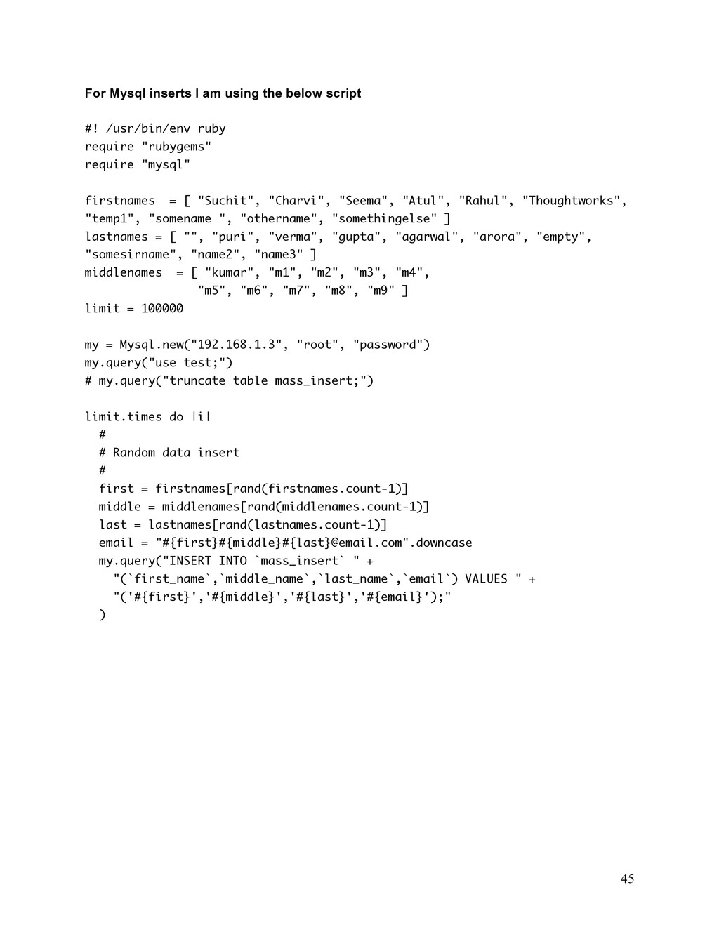
#! /usr/bin/env ruby require "rubygems" require "mysql" firstnames = [ "Suchit", "Charvi", "Seema", "Atul", "Rahul", "Thoughtworks", "temp1", "somename ", "othername", "somethingelse" ] lastnames = [ "", "puri", "verma", "gupta", "agarwal", "arora", "empty", "somesirname", "name2", "name3" ] middlenames = [ "kumar", "m1", "m2", "m3", "m4", "m5", "m6", "m7", "m8", "m9" ] limit = 100000 my = Mysql.new("192.168.1.3", "root", "password") my.query("use test;") # my.query("truncate table mass_insert;") limit.times do |i| # # Random data insert # first = firstnames[rand(firstnames.count-1)] middle = middlenames[rand(middlenames.count-1)] last = lastnames[rand(lastnames.count-1)] email = "#{first}#{middle}#{last}@email.com".downcase my.query("INSERT INTO `mass_insert` " + "(`first_name`,`middle_name`,`last_name`,`email`) VALUES " + "('#{first}','#{middle}','#{last}','#{email}');" )

46 Test Results Mongo Runs Pass 1: 6.70s user 1.06s
system 99% cpu 7.763 total Pass 2: 6.81s user 1.07s system 99% cpu 7.882 total Pass 3: 6.73s user 1.07s system 99% cpu 7.808 total An Average of 7.8176 seconds for 100000 records. MySQL Runs Pass 1: 1.67s user 2.29s system 18% cpu 21.544 total Pass 2: 1.60s user 2.37s system 18% cpu 21.678 total Pass 3: 1.66s user 2.40s system 17% cpu 23.185 total An Average of 22.1356 seconds for 10000 records. As you can see that the mongo inserts are approximately 3 times faster than the traditional MySQL. In spite of MongoDB having a global lock in its database the writes are much faster than the MySQL database The other interesting fact which came out was that the when the MySQL test ran the maximum CPU utilization was around 17 to 18% which means that there is still scope for improvement , and probably the MySQL ruby driver which we are using is not efficient enough to handle the so many writes.

47 Chapter 6 Summary In this whole paper we saw
3 different NoSql Databases, Amazon DynamoDB, Basho Riak and 10gen’s MongoDB. Out of these three databases, Amazon DynamoDB is the one, which was designed to suit the e- commerce application requirements at Amazon to server very high availability even under failure conditions. The research paper published by amazon [AMZ10] was the one that gave a direction to the industry the techniques mentioned in that paper specially the consistent hashing and vector clocks that gave way to many different other database in the industry specially RIAK , project Voldemort (from LinkedIn) and a few others. The database designed by amazon traded consistency in the cluster to availability, which meant that even under severe network and server failures the database will be able to server requests. The same concepts were used in the Riak database, which is an open source implementation of the concepts told in amazon dynamo research paper. The other good thing about Riak is that all the API work over http and as a result its integration with web projects is seamless and utilizes all the core concepts like caching. MongoDB is another set of NoSql database, which has concept of collections, which is a set of documents. MongoDB is the most popular NoSql option available today because of its query language being very similar to the existing SQL query language. MongoDB is also built to scale horizontally, which means that to get more throughputs you should add more MongoDB shards in the cluster.

48 Bibliography Books Pramod J Sadalage, Martin Fowler. NoSQL distilled
: a brief guide to the emerging world of polyglot persistence : Pearson Education (US). Kindle Edition. Kyle Banker. MongoDB in action, New York Manning Publication, 2012 Kristina Chodorow and Michael Dirolf. MongoDB: The Definitive Guide , 2010 Shashank Tiwari. Professional NoSql SCHOLARLY JOURNAL ARTICLES [10gen 01] 10gen, Inc: mongoDB. 2010. – http://www.mongodb.org [AMZ 10] Giuseppe DeCandia, Deniz Hastorun, Madan Jampani, Gunavardhan Kakulapati, Avinash Lakshman, Alex Pilchin, Swaminathan Sivasubramanian, Peter Vosshall and Werner Vogels. Dynamo: Amazon’s Highly Available Key-value Store [CAP01] Eric Brewer, "Towards Robust Distributed Systems", http://www.cs.berkeley.edu/%7Ebrewer/cs262b-2004/PODC-keynote.pdf [Jud09] Judd, Doug: Hypertable. June 2009. – Presentation at NoSQL meet-up in San Francisco on 2009-06-11.

NoSql Paper

NoSql Paper

More Decks by Suchit Puri

Other Decks in Technology

Featured

Transcript