株式会社TXP Medical リサーチチーム勉強会 "Double Machine Learning"

株式会社TXP Medicalのリサーチチームにおいて毎週月曜日夜20時半から行っている勉強会の一部資料です。 今回のテーマはDouble /Debiased Machine Learningで、アリゾナ経済大の原湖楠先生の解説になります。

※注：講義資料のため自己学習用にはなっていません。

Transcript

1. “Double/debiased machine learning for treatment and structural parameters” Chernozhukov et al. (2018) Konan Hara University of Arizona March 8, 2021
2. Today’s Presentation Vira Semenova’s UC Berkeley Econ 241C lecture note. Victor Chernozhukov’s 2016 U Chicago presentation. https://www.youtube.com/watch?v=eHOjmyoPCFU Konan Hara (Arizona) Double/debiased machine learning March 8, 2021 2 / 26
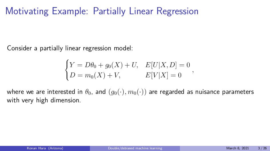
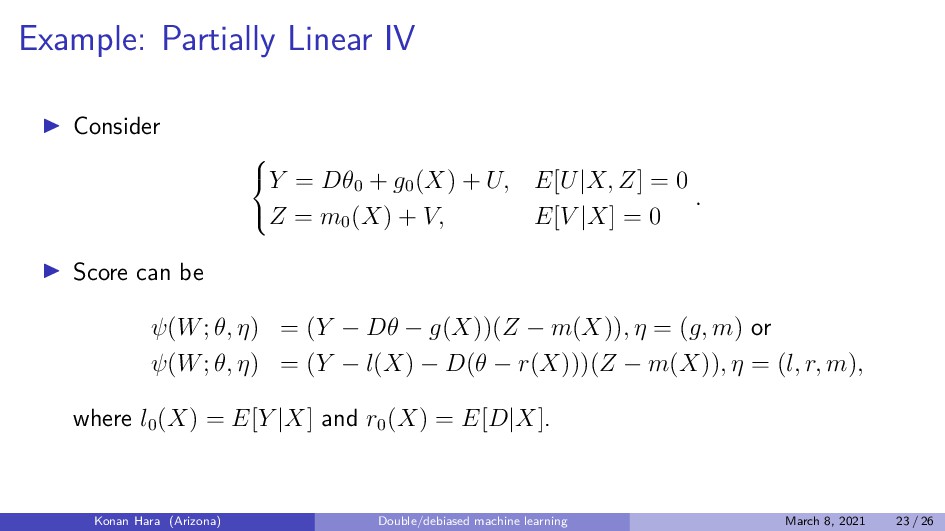
3. Motivating Example: Partially Linear Regression Consider a partially linear regression model:    Y = Dθ0 + g0 (X) + U, E[U|X, D] = 0 D = m0 (X) + V, E[V |X] = 0 , where we are interested in θ0 , and (g0 (·), m0 (·)) are regarded as nuisance parameters with very high dimension. Konan Hara (Arizona) Double/debiased machine learning March 8, 2021 3 / 26
4. Regularization Bias: Linear Regression Easy to get √ N-consistent θ0 if Y = Dθ0 + X β0 + U, E[U|X, D] = 0, β0 ∈ Rp, where p is small enough. Konan Hara (Arizona) Double/debiased machine learning March 8, 2021 4 / 26
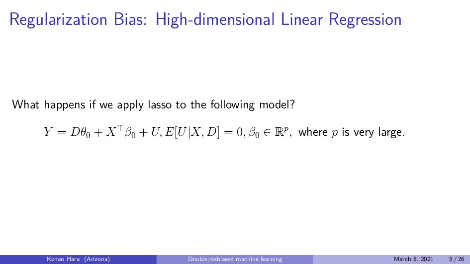
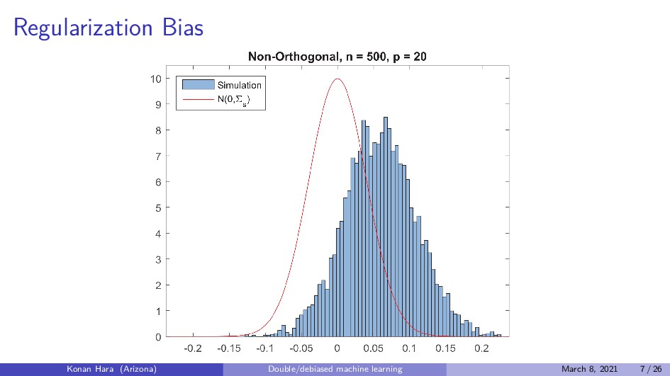
5. Regularization Bias: High-dimensional Linear Regression What happens if we apply lasso to the following model? Y = Dθ0 + X β0 + U, E[U|X, D] = 0, β0 ∈ Rp, where p is very large. Konan Hara (Arizona) Double/debiased machine learning March 8, 2021 5 / 26
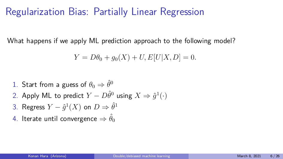
6. Regularization Bias: Partially Linear Regression What happens if we apply ML prediction approach to the following model? Y = Dθ0 + g0 (X) + U, E[U|X, D] = 0. 1. Start from a guess of θ0 ⇒ ˆ θ0 2. Apply ML to predict Y − Dˆ θ0 using X ⇒ ˆ g1(·) 3. Regress Y − ˆ g1(X) on D ⇒ ˆ θ1 4. Iterate until convergence ⇒ ˆ θ0 Konan Hara (Arizona) Double/debiased machine learning March 8, 2021 6 / 26
7. Regularization Bias Konan Hara (Arizona) Double/debiased machine learning March 8, 2021 7 / 26
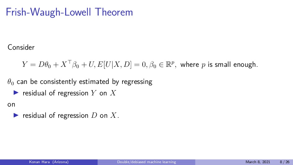
8. Frish-Waugh-Lowell Theorem Consider Y = Dθ0 + X β0 + U, E[U|X, D] = 0, β0 ∈ Rp, where p is small enough. θ0 can be consistently estimated by regressing residual of regression Y on X on residual of regression D on X. Konan Hara (Arizona) Double/debiased machine learning March 8, 2021 8 / 26
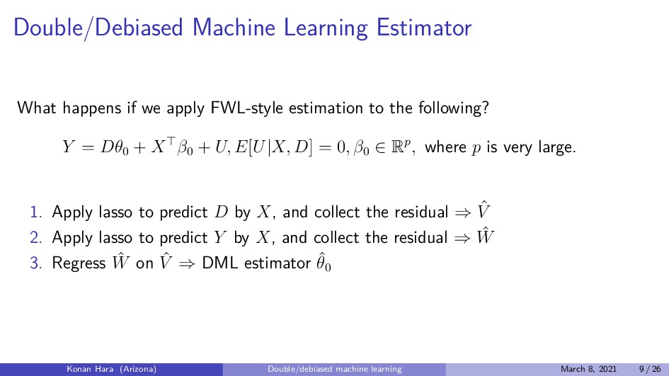
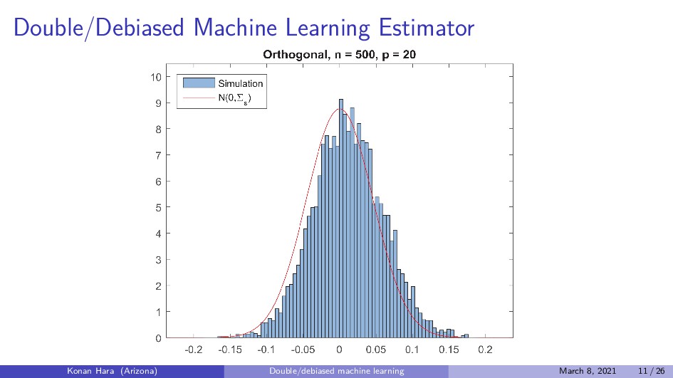
9. Double/Debiased Machine Learning Estimator What happens if we apply FWL-style estimation to the following? Y = Dθ0 + X β0 + U, E[U|X, D] = 0, β0 ∈ Rp, where p is very large. 1. Apply lasso to predict D by X, and collect the residual ⇒ ˆ V 2. Apply lasso to predict Y by X, and collect the residual ⇒ ˆ W 3. Regress ˆ W on ˆ V ⇒ DML estimator ˆ θ0 Konan Hara (Arizona) Double/debiased machine learning March 8, 2021 9 / 26
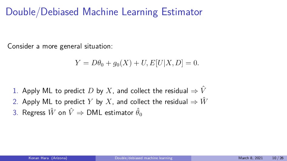
10. Double/Debiased Machine Learning Estimator Consider a more general situation: Y = Dθ0 + g0 (X) + U, E[U|X, D] = 0. 1. Apply ML to predict D by X, and collect the residual ⇒ ˆ V 2. Apply ML to predict Y by X, and collect the residual ⇒ ˆ W 3. Regress ˆ W on ˆ V ⇒ DML estimator ˆ θ0 Konan Hara (Arizona) Double/debiased machine learning March 8, 2021 10 / 26
11. Double/Debiased Machine Learning Estimator Konan Hara (Arizona) Double/debiased machine learning March 8, 2021 11 / 26
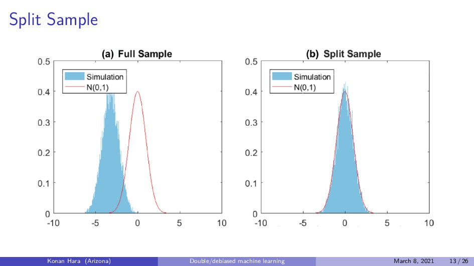
12. Split Sample We need to use independent sample sets for implementing 1. Estimation for residuals ˆ V and ˆ W 2. Regression ˆ W on ˆ V to get consistency. Konan Hara (Arizona) Double/debiased machine learning March 8, 2021 12 / 26
13. Split Sample Konan Hara (Arizona) Double/debiased machine learning March 8, 2021 13 / 26
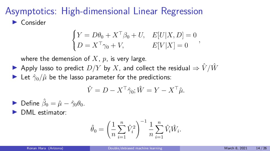
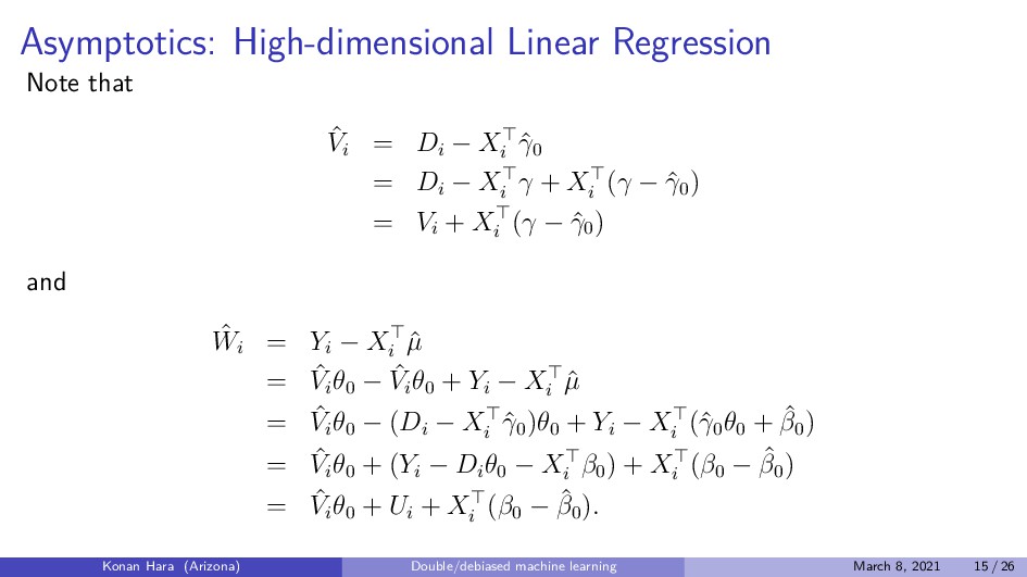
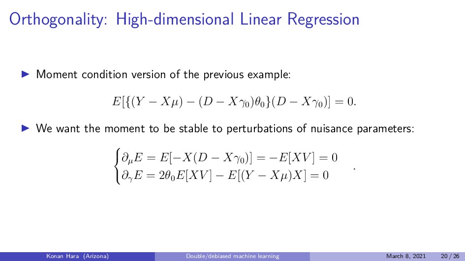
14. Asymptotics: High-dimensional Linear Regression Consider    Y = Dθ0 + X β0 + U, E[U|X, D] = 0 D = X γ0 + V, E[V |X] = 0 , where the demension of X, p, is very large. Apply lasso to predict D/Y by X, and collect the residual ⇒ ˆ V / ˆ W Let ˆ γ0 /ˆ µ be the lasso parameter for the predictions: ˆ V = D − X ˆ γ0 ; ˆ W = Y − X ˆ µ. Define ˆ β0 = ˆ µ − ˆ γ0 θ0 . DML estimator: ˆ θ0 = 1 n n i=1 ˆ V 2 i −1 1 n n i=1 ˆ Vi ˆ Wi . Konan Hara (Arizona) Double/debiased machine learning March 8, 2021 14 / 26
15. Asymptotics: High-dimensional Linear Regression Note that ˆ Vi = Di − Xi ˆ γ0 = Di − Xi γ + Xi (γ − ˆ γ0 ) = Vi + Xi (γ − ˆ γ0 ) and ˆ Wi = Yi − Xi ˆ µ = ˆ Vi θ0 − ˆ Vi θ0 + Yi − Xi ˆ µ = ˆ Vi θ0 − (Di − Xi ˆ γ0 )θ0 + Yi − Xi (ˆ γ0 θ0 + ˆ β0 ) = ˆ Vi θ0 + (Yi − Di θ0 − Xi β0 ) + Xi (β0 − ˆ β0 ) = ˆ Vi θ0 + Ui + Xi (β0 − ˆ β0 ). Konan Hara (Arizona) Double/debiased machine learning March 8, 2021 15 / 26
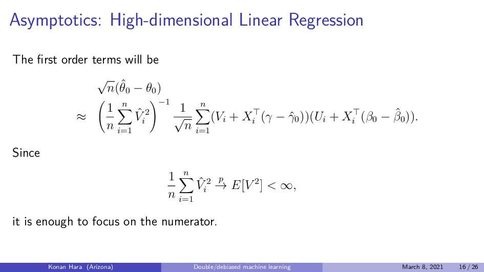
16. Asymptotics: High-dimensional Linear Regression The first order terms will be √ n(ˆ θ0 − θ0 ) ≈ 1 n n i=1 ˆ V 2 i −1 1 √ n n i=1 (Vi + Xi (γ − ˆ γ0 ))(Ui + Xi (β0 − ˆ β0 )). Since 1 n n i=1 ˆ V 2 i p → E[V 2] < ∞, it is enough to focus on the numerator. Konan Hara (Arizona) Double/debiased machine learning March 8, 2021 16 / 26
17. Asymptotics: High-dimensional Linear Regression Decomposition of 1 √ n n i=1 (Vi + Xi (γ − ˆ γ0 ))(Ui + Xi (β0 − ˆ β0 )): 1 √ n n i=1 (Vi + Xi (γ − ˆ γ0 ))Ui a ∼ N(0, Σ) standard CLT argument with ˆ γ0 ⊥ ⊥ U 1 √ n n i=1 (Xi (γ − ˆ γ0 ))(Xi (β0 − ˆ β0 )) ≤ 1 √ n n i=1 Xi Xi γ − ˆ γ0 2 β0 − ˆ β0 2 1 √ n n i=1 Xi Xi ≈ 1 √ n ∗ n ∗ O(1) = O(n1/2) want γ − ˆ γ0 2 and β0 − ˆ β0 2 ≈ o(n−1/4) ≈ O(n1/2) ∗ o(n−1/4) ∗ o(n−1/4) = o(1) 1 √ n n i=1 Vi (Xi (β0 − ˆ β0 )) use sample splitting to attain ˆ β0 ⊥ ⊥ V Konan Hara (Arizona) Double/debiased machine learning March 8, 2021 17 / 26
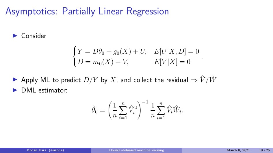
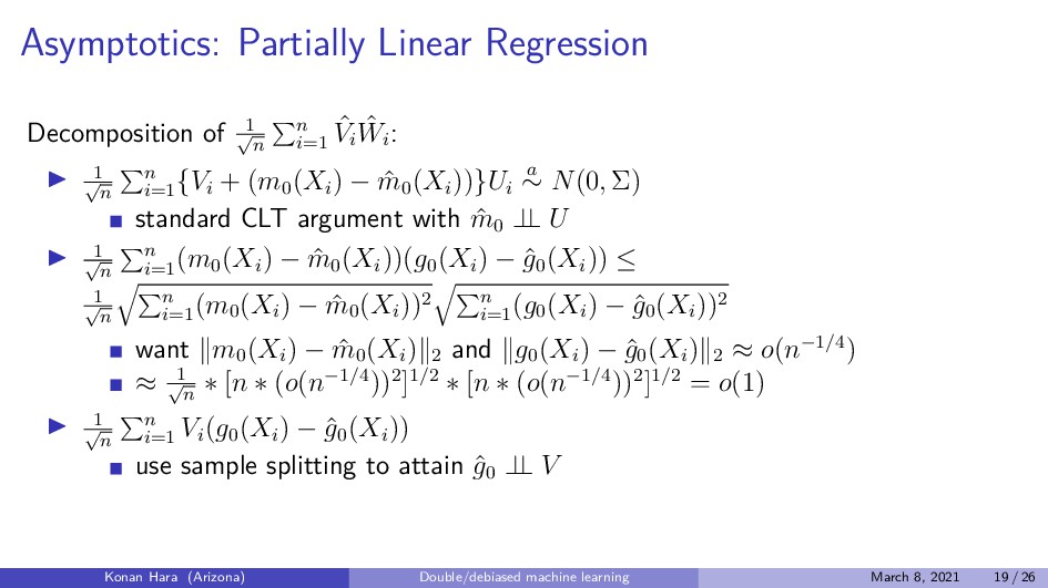
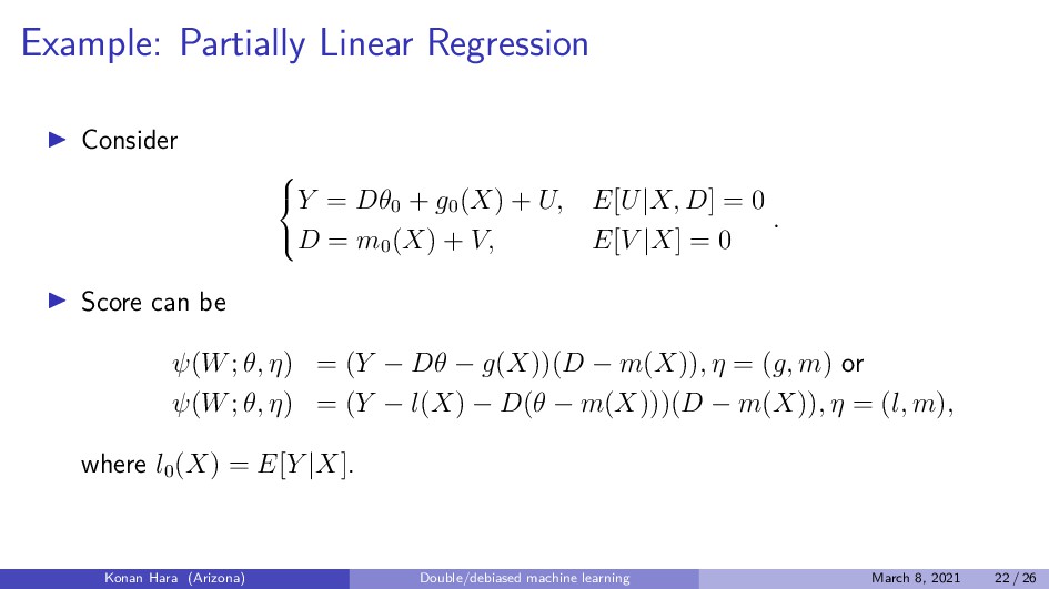
18. Asymptotics: Partially Linear Regression Consider    Y = Dθ0 + g0 (X) + U, E[U|X, D] = 0 D = m0 (X) + V, E[V |X] = 0 . Apply ML to predict D/Y by X, and collect the residual ⇒ ˆ V / ˆ W DML estimator: ˆ θ0 = 1 n n i=1 ˆ V 2 i −1 1 n n i=1 ˆ Vi ˆ Wi . Konan Hara (Arizona) Double/debiased machine learning March 8, 2021 18 / 26
19. Asymptotics: Partially Linear Regression Decomposition of 1 √ n n i=1 ˆ Vi ˆ Wi : 1 √ n n i=1 {Vi + (m0 (Xi ) − ˆ m0 (Xi ))}Ui a ∼ N(0, Σ) standard CLT argument with ˆ m0 ⊥ ⊥ U 1 √ n n i=1 (m0 (Xi ) − ˆ m0 (Xi ))(g0 (Xi ) − ˆ g0 (Xi )) ≤ 1 √ n n i=1 (m0 (Xi ) − ˆ m0 (Xi ))2 n i=1 (g0 (Xi ) − ˆ g0 (Xi ))2 want m0 (Xi ) − ˆ m0 (Xi ) 2 and g0 (Xi ) − ˆ g0 (Xi ) 2 ≈ o(n−1/4) ≈ 1 √ n ∗ [n ∗ (o(n−1/4))2]1/2 ∗ [n ∗ (o(n−1/4))2]1/2 = o(1) 1 √ n n i=1 Vi (g0 (Xi ) − ˆ g0 (Xi )) use sample splitting to attain ˆ g0 ⊥ ⊥ V Konan Hara (Arizona) Double/debiased machine learning March 8, 2021 19 / 26
20. Orthogonality: High-dimensional Linear Regression Moment condition version of the previous example: E[{(Y − Xµ) − (D − Xγ0 )θ0 }(D − Xγ0 )] = 0. We want the moment to be stable to perturbations of nuisance parameters:    ∂µ E = E[−X(D − Xγ0 )] = −E[XV ] = 0 ∂γ E = 2θ0 E[XV ] − E[(Y − Xµ)X] = 0 . Konan Hara (Arizona) Double/debiased machine learning March 8, 2021 20 / 26
21. Orthogonality: Non-linear Moment Condition General non-linear moment condition: E[ψ(W; θ0 , η0 )] = 0. In previous examples, W = (Y, D, X) and η0 = (β0 , γ0 ) or (g0 , m0 ). Orthogonality condition: ∂η E[ψ(W; θ0 , η0 )] = 0. Konan Hara (Arizona) Double/debiased machine learning March 8, 2021 21 / 26
22. Example: Partially Linear Regression Consider    Y = Dθ0 + g0 (X) + U, E[U|X, D] = 0 D = m0 (X) + V, E[V |X] = 0 . Score can be ψ(W; θ, η) = (Y − Dθ − g(X))(D − m(X)), η = (g, m) or ψ(W; θ, η) = (Y − l(X) − D(θ − m(X)))(D − m(X)), η = (l, m), where l0 (X) = E[Y |X]. Konan Hara (Arizona) Double/debiased machine learning March 8, 2021 22 / 26
23. Example: Partially Linear IV Consider    Y = Dθ0 + g0 (X) + U, E[U|X, Z] = 0 Z = m0 (X) + V, E[V |X] = 0 . Score can be ψ(W; θ, η) = (Y − Dθ − g(X))(Z − m(X)), η = (g, m) or ψ(W; θ, η) = (Y − l(X) − D(θ − r(X)))(Z − m(X)), η = (l, r, m), where l0 (X) = E[Y |X] and r0 (X) = E[D|X]. Konan Hara (Arizona) Double/debiased machine learning March 8, 2021 23 / 26
24. Example: ATE Consider    Y = g0 (D, X) + U, E[U|X, D] = 0 D = m0 (X) + V, E[V |X] = 0 . Want to estimate ATE: θ0 = E[g0 (1, X) − g0 (0, X)]. Score can be ψ(W; θ, η) = (g(1, X) − g(0, X)) + D(Y − g(1, X)) m(X) − (1 − D)(Y − g(0, X)) 1 − m(X) − θ, where η = (g, m). Konan Hara (Arizona) Double/debiased machine learning March 8, 2021 24 / 26
25. Example: ATTE Consider    Y = g0 (D, X) + U, E[U|X, D] = 0 D = m0 (X) + V, E[V |X] = 0 . Want to estimate ATTE: θ0 = E[g0 (1, X) − g0 (0, X)|D = 1]. Score can be ψ(W; θ, η) = D(Y − g(0, X)) − m(X)(1 − D)(Y − g(0, X)) 1 − m(X) − Dθ, where η = (g(0, ·), m). Konan Hara (Arizona) Double/debiased machine learning March 8, 2021 25 / 26
26. Example: LATE Consider        Y = µ0 (Z, X) + U, E[U|Z, X] = 0 D = m0 (Z, X) + V, E[V |Z, X] = 0 Z = p0 (X) + ζ, E[ζ|X] = 0 . Want to estimate LATE: θ0 = E[µ0 (1, X) − µ0 (0, X)] E[m0 (1, X) − m0 (0, X)] . Score can be (µ(1, X) − µ(0, X)) + Z(Y − µ(1, X)) p(X) − (1 − Z)(Y − µ(0, X)) 1 − p(X) − (m(1, X) − m(0, X)) + Z(D − m(1, X)) p(X) − (1 − Z)(D − m(0, X)) 1 − p(X) θ. Konan Hara (Arizona) Double/debiased machine learning March 8, 2021 26 / 26