On the edge: State tomography, boundaries, and model selection

A talk I presented at the Center for Quantum Information and Control to provide an update on my research progress.

Transcript

1. ON THE EDGE: STATE TOMOGRAPHY, BOUNDARIES, AND MODEL SELECTION Travis L Scholten Center for Computing Research Sandia National Labs CQuIC Talk University of New Mexico 2015 December 2 Sandia National Laboratories is a multi-program laboratory managed and operated by Sandia Corporation, a wholly owned subsidiary of Lockheed Martin Corporation, for the U.S. Department of Energy’s National Nuclear Security Administration under contract DE-AC04-94AL85000. CCR Center for Computing Research 59
2. I am interested in tomography, the characterization of quantum systems. 58
3. Characterizing a system means estimating/ inferring something about it. ˆ ⇢ Tomography is a statistical inference problem Estimator (Things with hats) (Experiment) (Inference) Data Estimates POVM {Ej } 57
4. The “best” estimator is very accurate. Many measures of accuracy: We seek high accuracy relative to an unknown truth. Quantum Fidelity Relative Entropy Trace Distance Hilbert-Schmidt Distance 56
5. The “ideal” estimator would be very accurate… and would not fit noise in the data. “Ideal” impossible to achieve! 55
6. We do not have truth, only data. How do we be accurate and fit well? Model selection. Truth Data 54 Model selection: Find best model Fit parameters in model
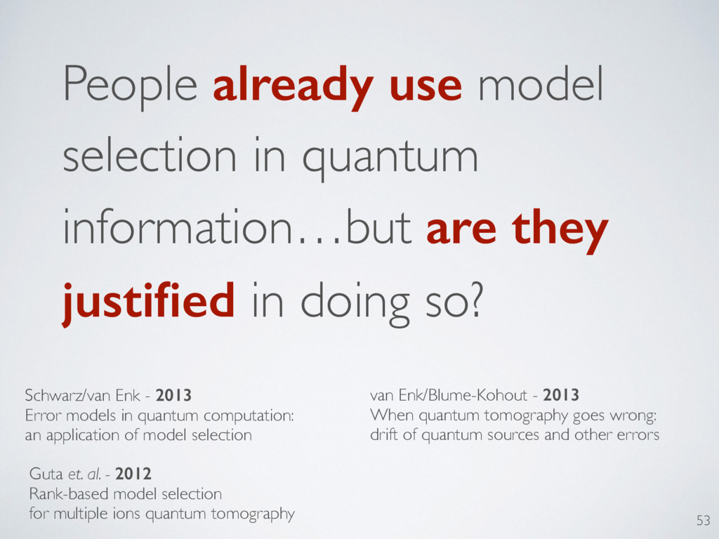
7. People already use model selection in quantum information…but are they justified in doing so? Schwarz/van Enk - 2013 Error models in quantum computation: an application of model selection Guta et. al. - 2012 Rank-based model selection
 for multiple ions quantum tomography van Enk/Blume-Kohout - 2013 When quantum tomography goes wrong:
 drift of quantum sources and other errors 53
8. Model selection techniques currently used in quantum tomography may have problems. Such as loglikelihood ratio tests, or Akaike’s AIC.
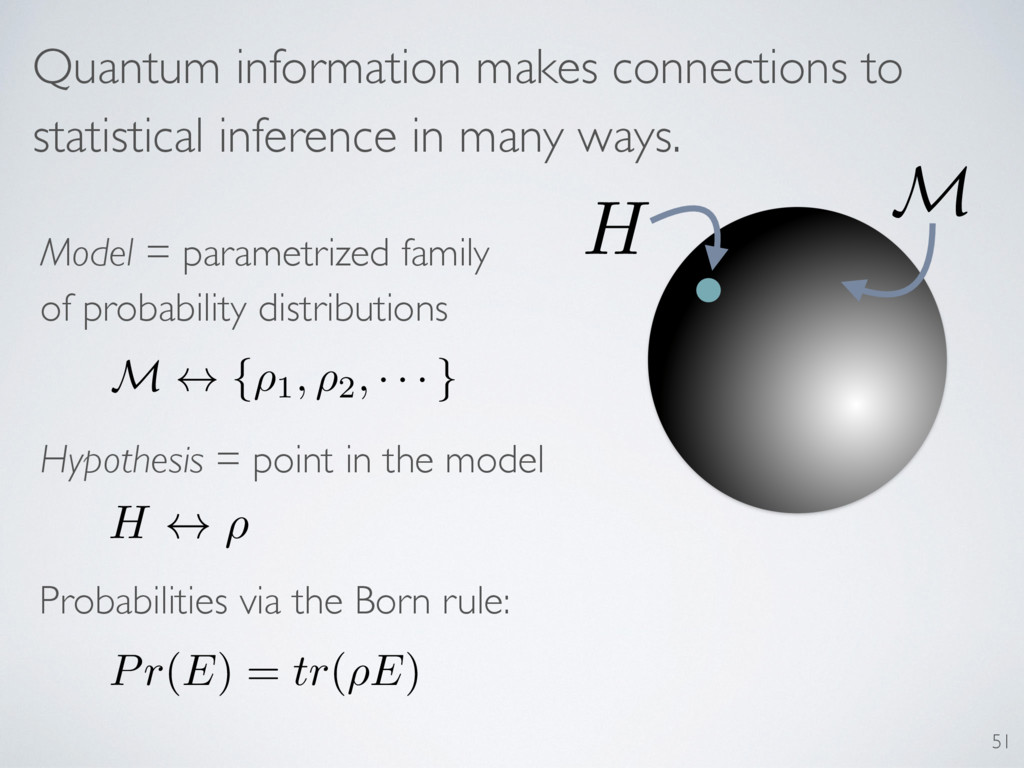
9. Quantum information makes connections to statistical inference in many ways. Model = parametrized family
 of probability distributions Probabilities via the Born rule: Pr(E) = tr(⇢E) Hypothesis = point in the model M H 51 H $ ⇢ M $ {⇢1, ⇢2, · · · }
10. Given some data, plausibility of a model/hypothesis
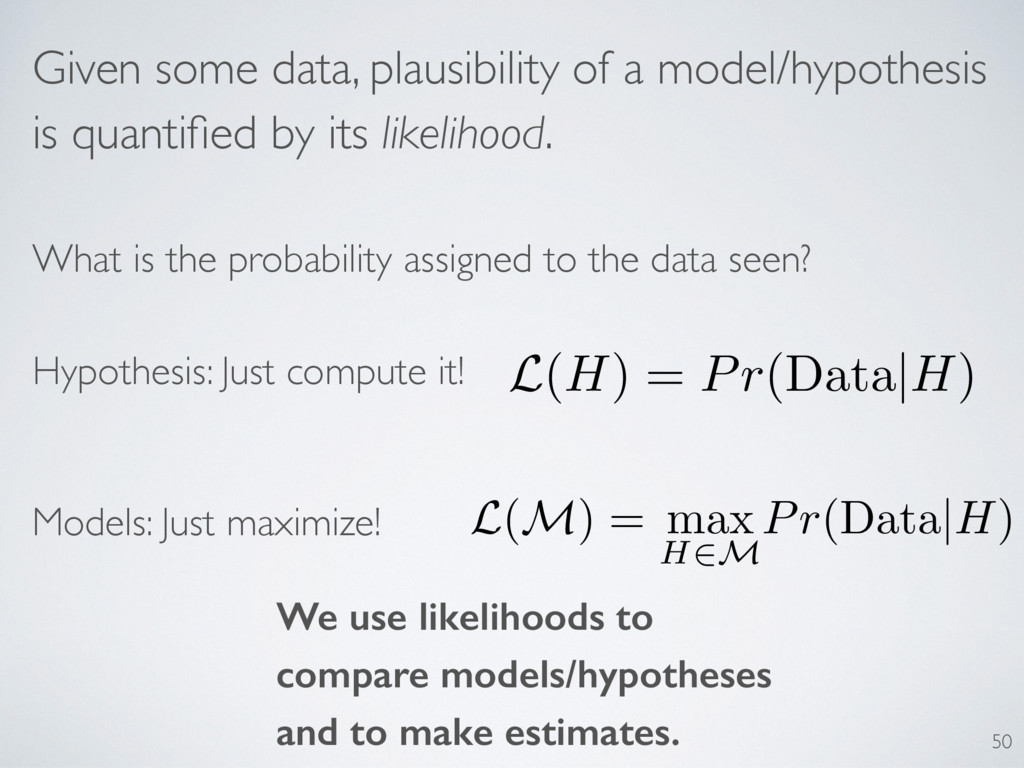
 is quantified by its likelihood. What is the probability assigned to the data seen? L(H) = Pr(Data|H) Hypothesis: Just compute it! L ( M ) = max H2M Pr (Data |H ) Models: Just maximize! We use likelihoods to
 compare models/hypotheses
 and to make estimates. 50
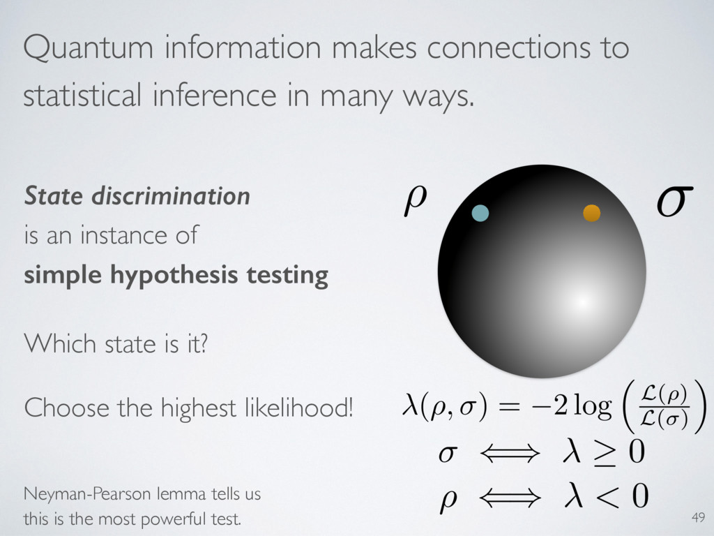
11. Quantum information makes connections to statistical inference in many ways. State discrimination
 is an instance of
 simple hypothesis testing Which state is it? ⇢ Neyman-Pearson lemma tells us
 this is the most powerful test. ( ⇢, ) = 2 log ⇣ L(⇢) L( ) ⌘ () 0 Choose the highest likelihood! 49 ⇢ () < 0
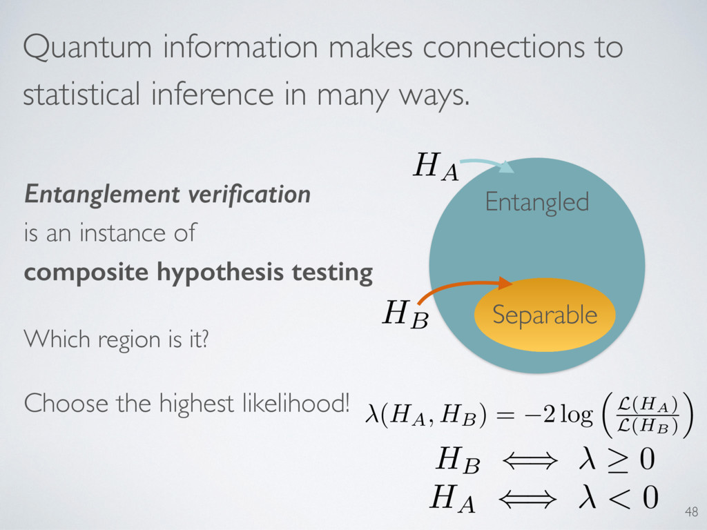
12. Quantum information makes connections to statistical inference in many ways. Entanglement verification
 is an instance of
 composite hypothesis testing Which region is it? Separable Entangled 48 Choose the highest likelihood! ( HA , HB ) = 2 log ⇣ L(HA) L(HB) ⌘ HB () 0 HA () < 0 HA HB
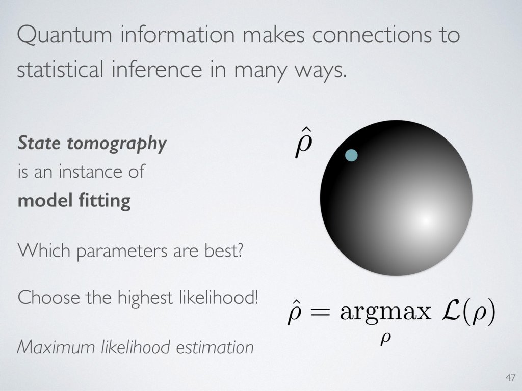
13. Quantum information makes connections to statistical inference in many ways. State tomography
 is an instance of
 model fitting Which parameters are best? Maximum likelihood estimation ˆ ⇢ ˆ ⇢ = argmax ⇢ L ( ⇢ ) 47 Choose the highest likelihood!
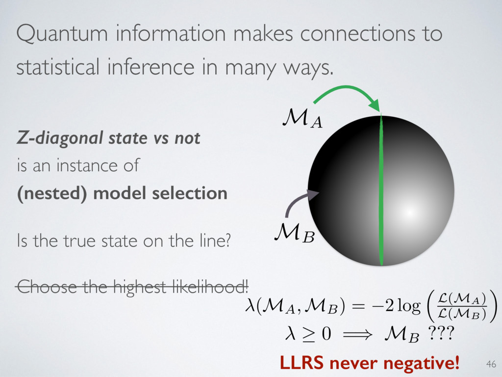
14. Quantum information makes connections to statistical inference in many ways. Z-diagonal state vs not
 is an instance of
 (nested) model selection Is the true state on the line? 0 =) MB ??? LLRS never negative! ( MA, MB) = 2 log ⇣ L(MA) L(MB) ⌘ MA MB 46 Choose the highest likelihood!
15. How will we investigate
 model selection
 in state tomography?
16. I am studying a paradigmatic problem: tomography of continuous-variable systems. Optical modes of light… …as Wigner functions
 or density matrices. ˆ ⇢ 44
17. The models I consider are subspaces of an infinite-dimensional Hilbert space. |0i |1i |2i |d 1i Other models are possible (e.g., by rank). Hd = Span (|0i, |1i, · · · |d 1i) Md = {⇢ | ⇢ 2 B(Hd), Tr(⇢) = 1, ⇢ 0} Models based on 
 low-energy approximation
 and smoothness of 
 Wigner function. 43
18. The models I consider are nested inside one another. Md ⇢ Md+1 How can we use likelihoods
 to compare them? We have to tackle
 nested model selection 42 |0i |1i |2i |d 1i
19. We rethink using the LLRS for nested model selection, based on its null expected value. N h i Md Md0 ( Md, Md0 ) = 2 log ⇣ L(Md) L(Md0 ) ⌘ 41 Case One: Smaller Model is False
20. We rethink using the LLRS for nested model selection, based on its null expected value. Case Two: Both Models True (Null case) N h i Md Md0 40 ( Md, Md0 ) = 2 log ⇣ L(Md) L(Md0 ) ⌘
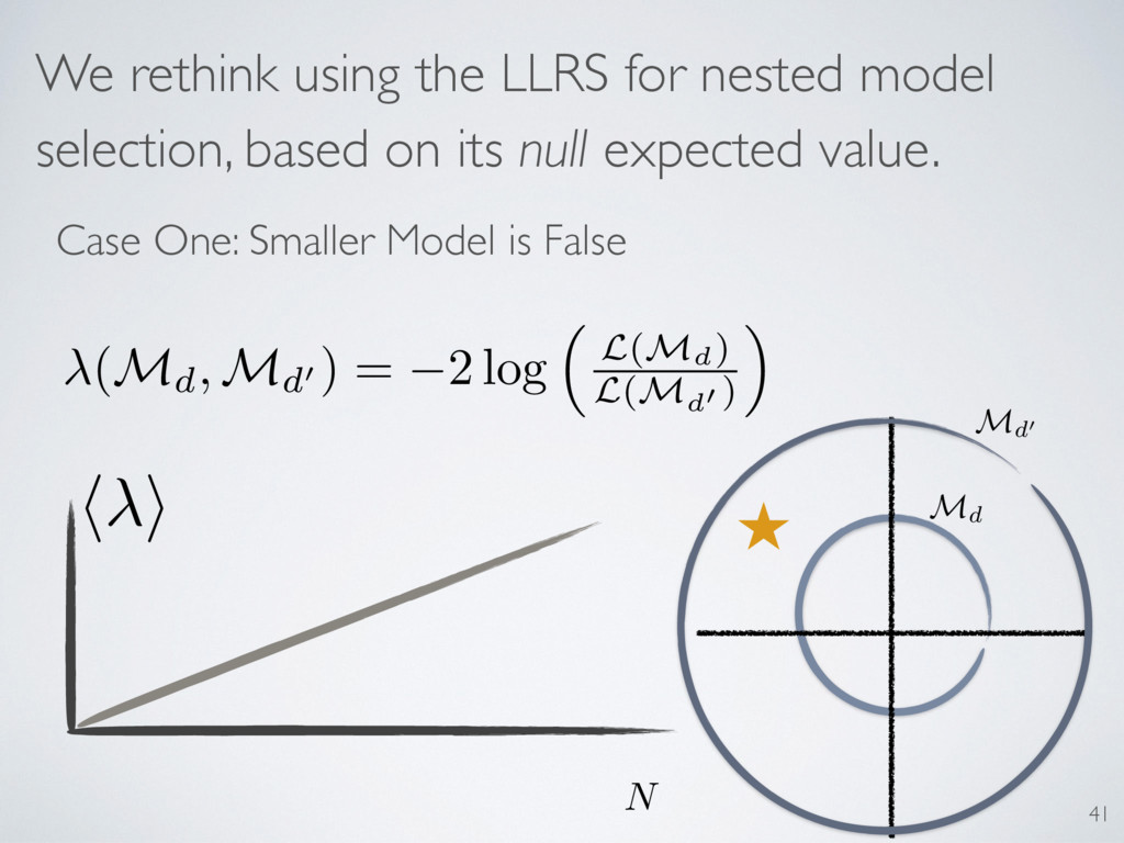
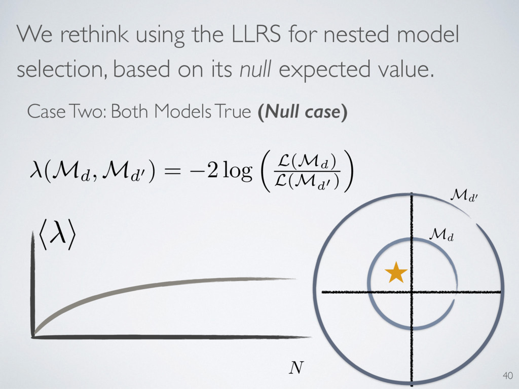
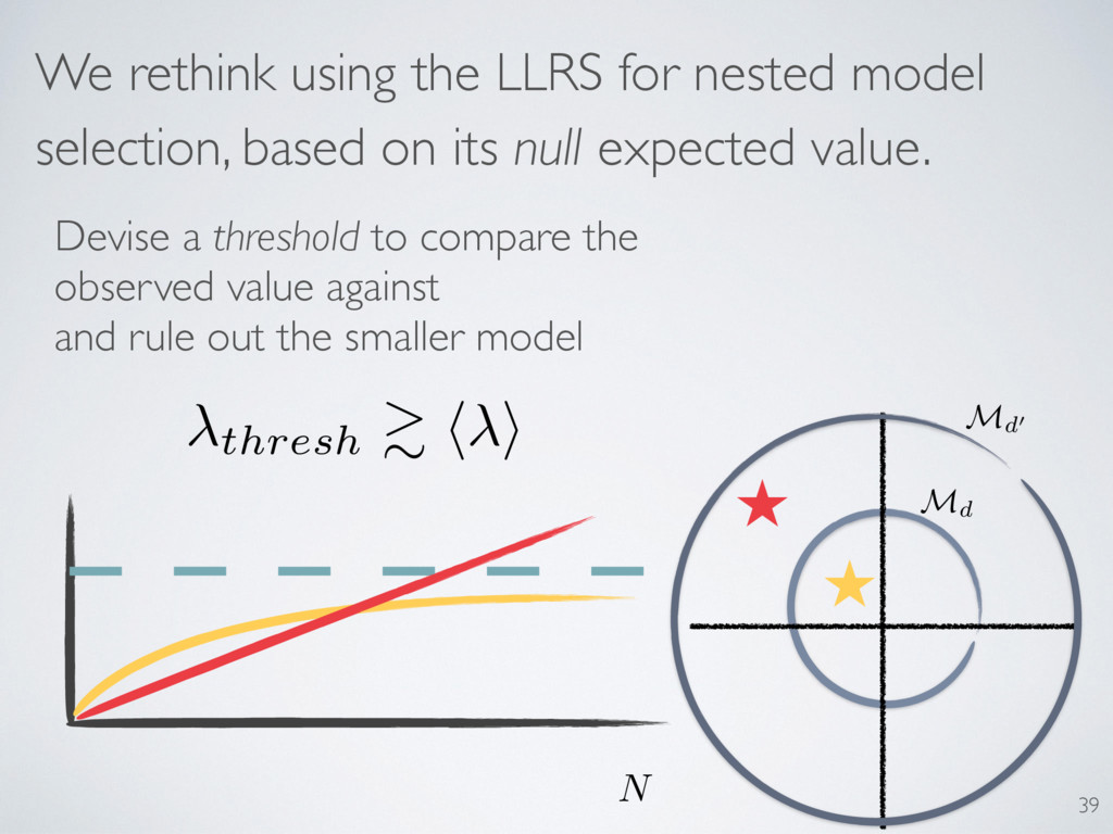
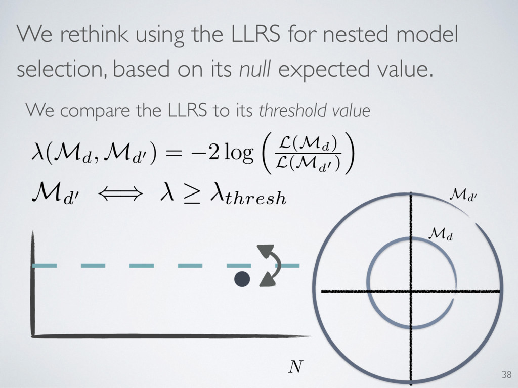
21. N Md Md0 39 We rethink using the LLRS for nested model selection, based on its null expected value. Devise a threshold to compare the observed value against
 and rule out the smaller model thresh & h i
22. We compare the LLRS to its threshold value ( Md, Md0 ) = 2 log ⇣ L(Md) L(Md0 ) ⌘ 38 We rethink using the LLRS for nested model selection, based on its null expected value. Md0 () thresh Md Md0 N
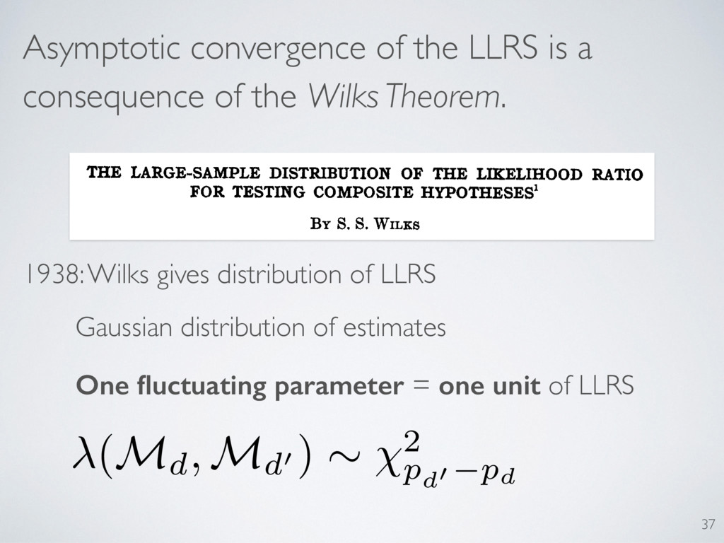
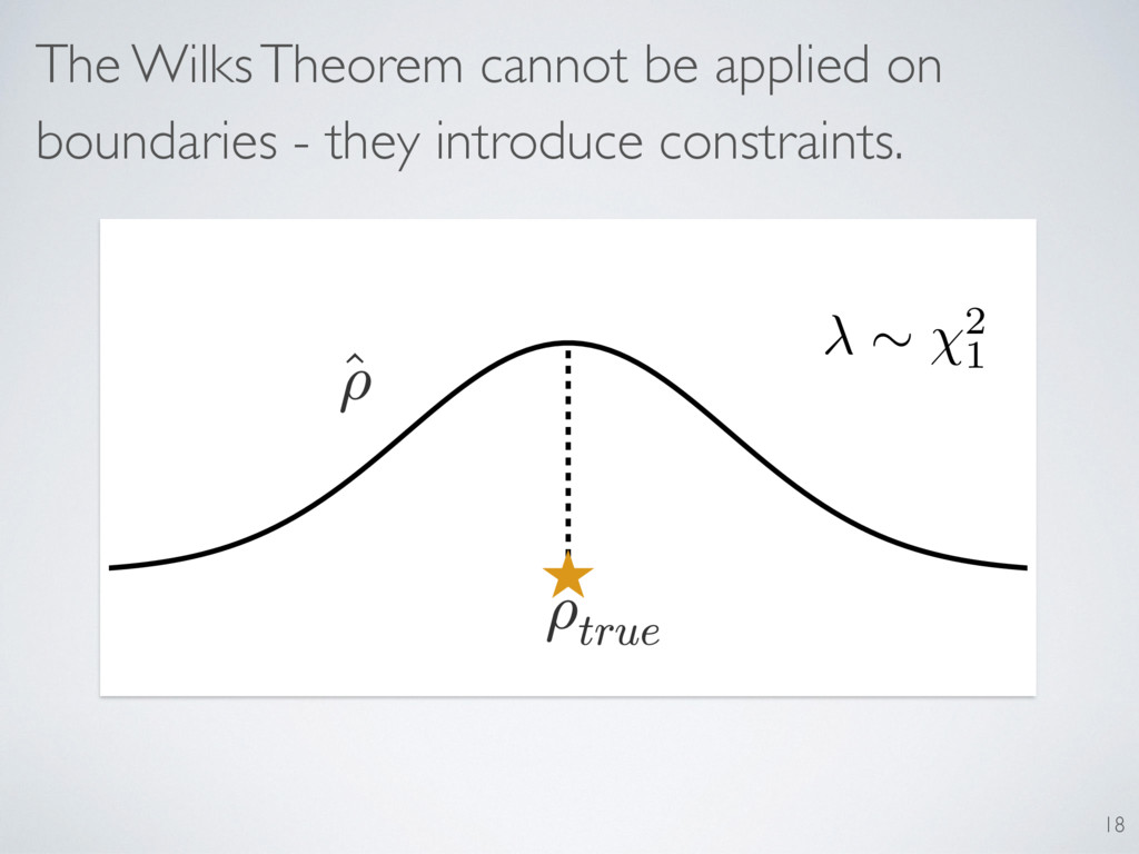
23. Asymptotic convergence of the LLRS is a consequence of the Wilks Theorem. 1938: Wilks gives distribution of LLRS (Md, Md0 ) ⇠ 2 pd0 pd 37 Gaussian distribution of estimates One fluctuating parameter = one unit of LLRS
24. Another model selection technique
 relies on this result. Information criteria trade off between
 fitting data well and having high accuracy Use of Akaike’s AIC is common Relies on Wilks Theorem
 (bias of estimator of KL divergence) My work helps us create a quantum information criterion 36
25. We now have potential tools for nested model selection
 in tomography.
 How do they perform?
26. I performed a Monte Carlo study of the LLRS and its behavior. Studied: - 17 true states (supported on low-energy subspace) 34
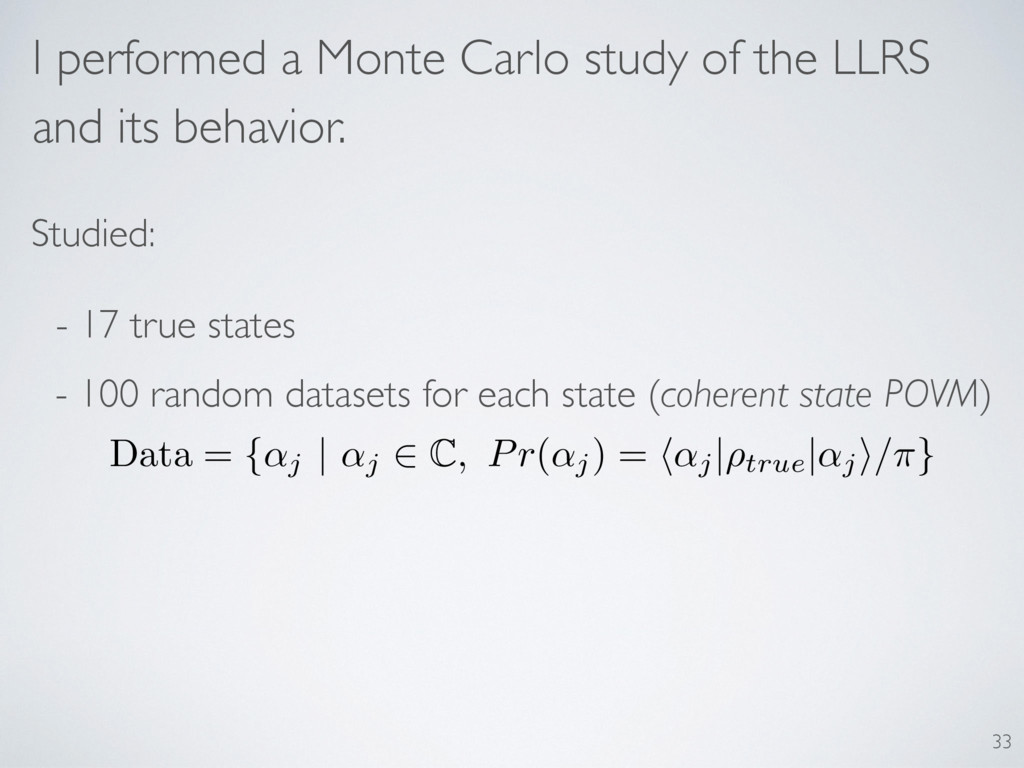
27. I performed a Monte Carlo study of the LLRS and its behavior. Studied: - 17 true states - 100 random datasets for each state (coherent state POVM) Data = {↵j | ↵j 2 C, Pr(↵j) = h↵j |⇢true |↵j i/⇡} 33
28. I performed a Monte Carlo study of the LLRS and its behavior. Studied: - 17 true states - 100 random datasets for each state (coherent state POVM) 32 - 10K to 100K samples for each dataset
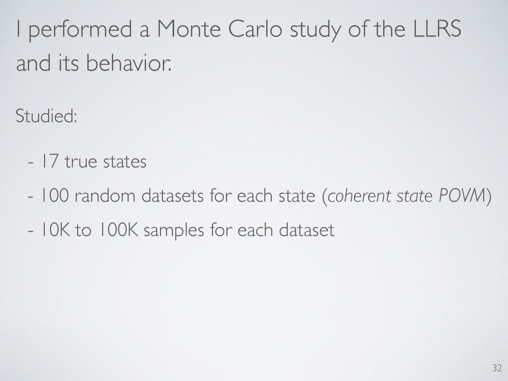
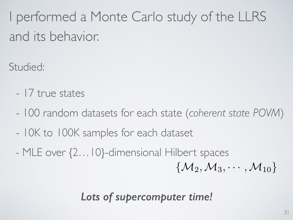
29. I performed a Monte Carlo study of the LLRS and its behavior. Studied: - 17 true states - 100 random datasets for each state (coherent state POVM) 31 - 10K to 100K samples for each dataset - MLE over {2…10}-dimensional Hilbert spaces {M2, M3, · · · , M10 } Lots of supercomputer time!
30. The results were puzzling.
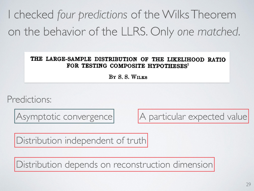
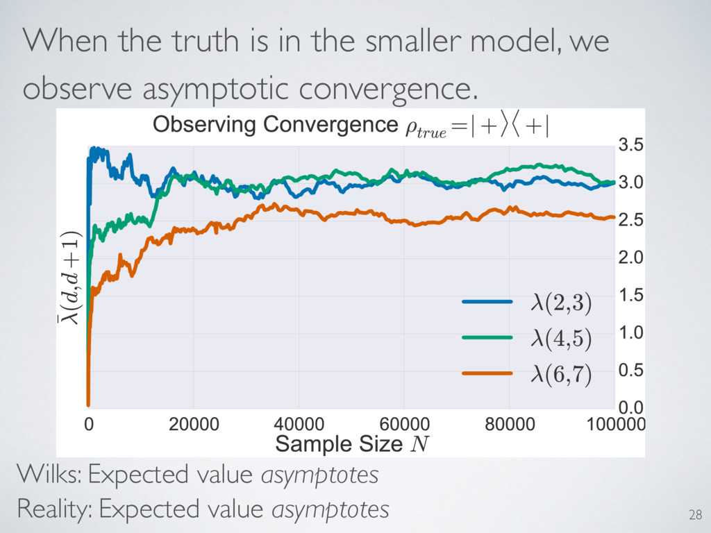
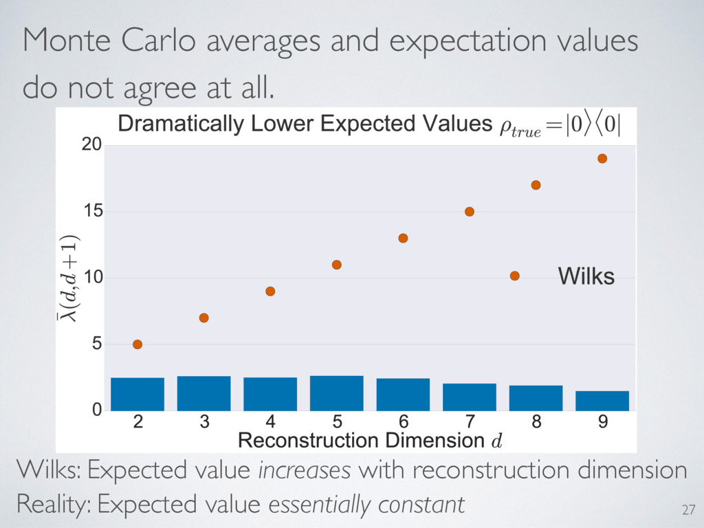
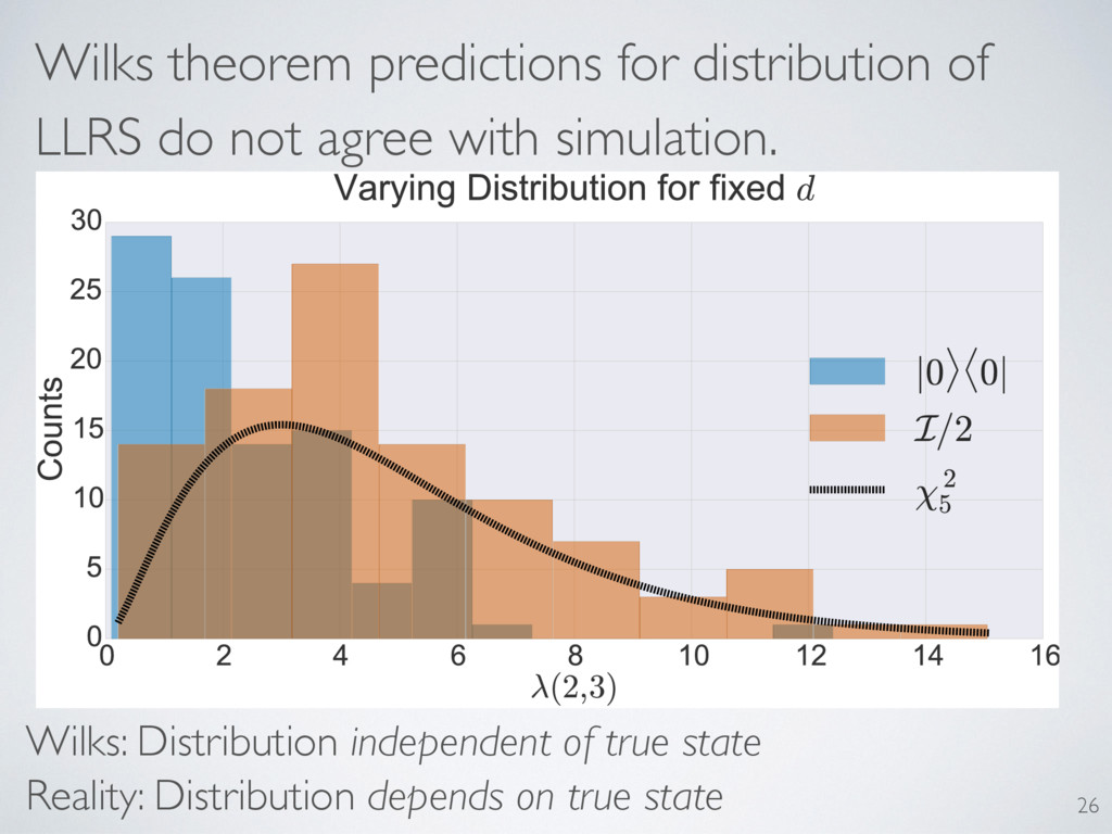
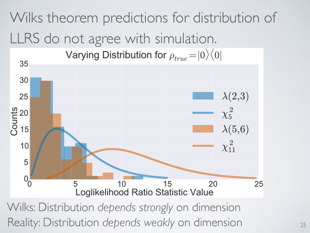
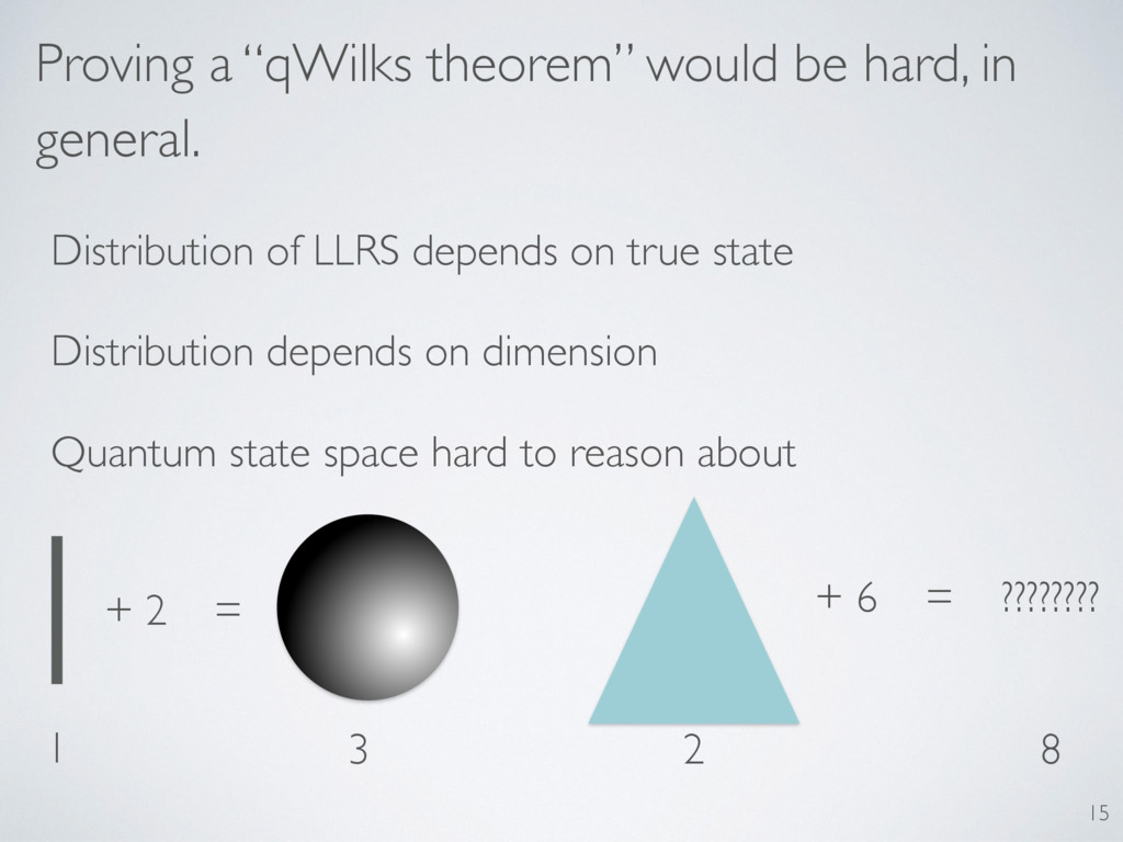
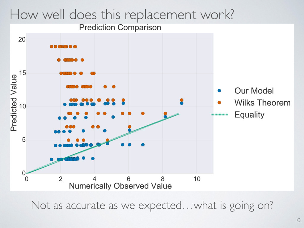
31. I checked four predictions of the Wilks Theorem on the behavior of the LLRS. Only one matched. Predictions: Asymptotic convergence Distribution independent of truth A particular expected value Distribution depends on reconstruction dimension 29
32. When the truth is in the smaller model, we observe asymptotic convergence. 28 Wilks: Expected value asymptotes Reality: Expected value asymptotes
33. Monte Carlo averages and expectation values do not agree at all. Wilks: Expected value increases with reconstruction dimension 27 Reality: Expected value essentially constant
34. Wilks theorem predictions for distribution of LLRS do not agree with simulation. Wilks: Distribution independent of true state 26 Reality: Distribution depends on true state
35. Wilks theorem predictions for distribution of LLRS do not agree with simulation. Wilks: Distribution depends strongly on dimension 25 Reality: Distribution depends weakly on dimension
36. Theorems are not “wrong”,
 only “not applicable”. Why does the Wilks Theorem not apply?
37. State tomography is
 on the edge. Let’s see why.
38. The first edge is the positivity constraint. This shows up a lot in quantum information. ˆ ⇢ 0 ˆ ⇢  0 22
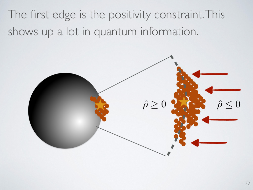
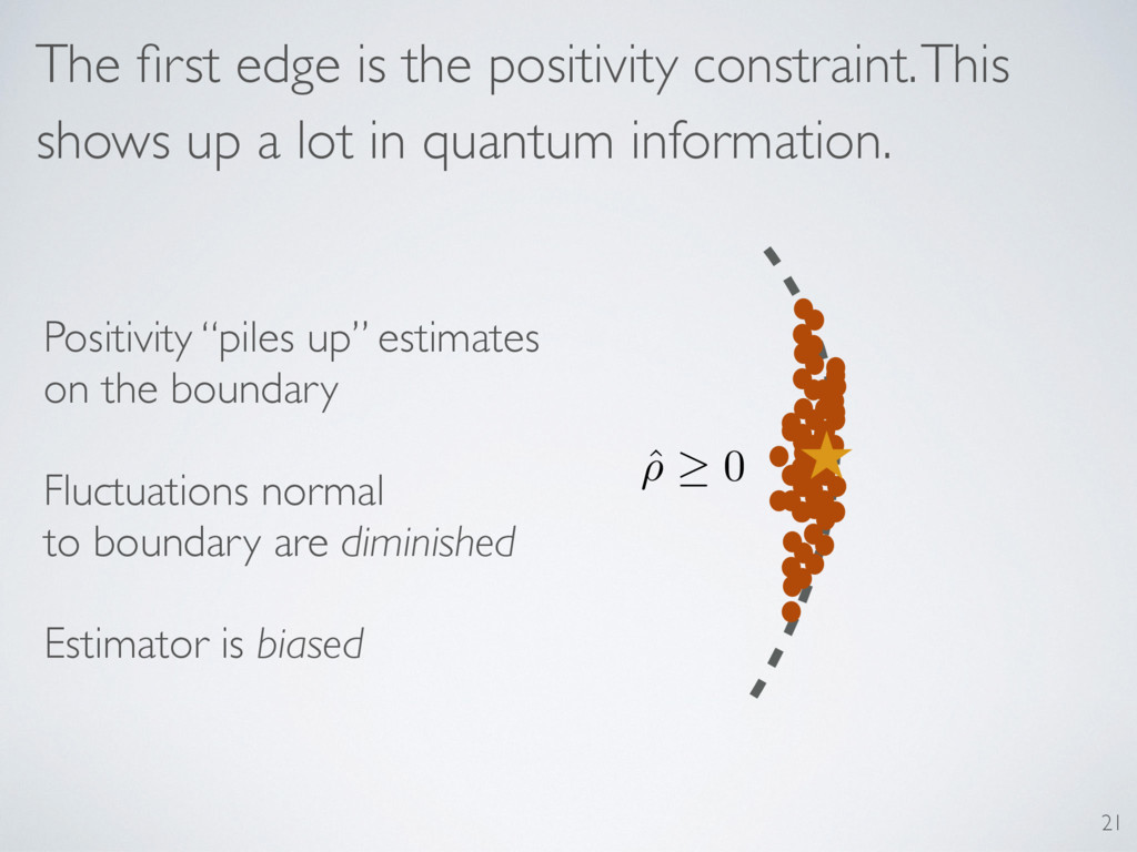
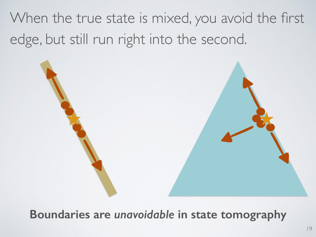
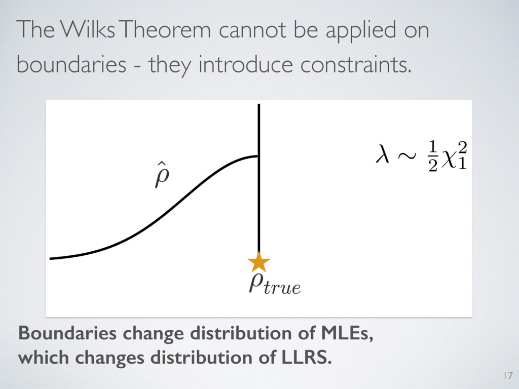
39. The first edge is the positivity constraint. This shows up a lot in quantum information. Positivity “piles up” estimates
 on the boundary ! Fluctuations normal
 to boundary are diminished ! Estimator is biased ˆ ⇢ 0 21
40. The second edge is that the models I use nest on the boundary of one another. ˆ ⇢ = 0 B B B @ ⇢00 ⇢01 ⇢02 · · · ⇢10 ⇢11 ⇢12 · · · ⇢20 ⇢21 ⇢22 · · · . . . . . . . . . ... 1 C C C A 20
41. When the true state is mixed, you avoid the first edge, but still run right into the second. 19 Boundaries are unavoidable in state tomography
42. The Wilks Theorem cannot be applied on boundaries - they introduce constraints. 18 ⇠ 2 1
43. The Wilks Theorem cannot be applied on boundaries - they introduce constraints. Boundaries change distribution of MLEs,
 which changes distribution of LLRS. 17 ⇠ 1 2 2 1
44. State tomography is
 on the edge. So must our
 model selection be.
45. Proving a “qWilks theorem” would be hard, in general. Distribution of LLRS depends on true state Quantum state space hard to reason about Distribution depends on dimension + 6 3 15 1 + 2 = = ???????? 2 8
46. Can we find a replacement for the Wilks theorem which respects boundaries? 14 Let’s talk about work in progress.
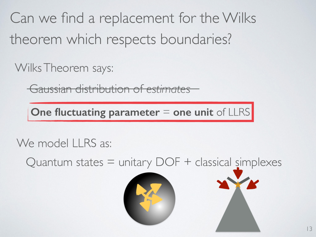
47. Can we find a replacement for the Wilks theorem which respects boundaries? Quantum states = unitary DOF + classical simplexes 13 Gaussian distribution of estimates Wilks Theorem says: We model LLRS as: One fluctuating parameter = one unit of LLRS
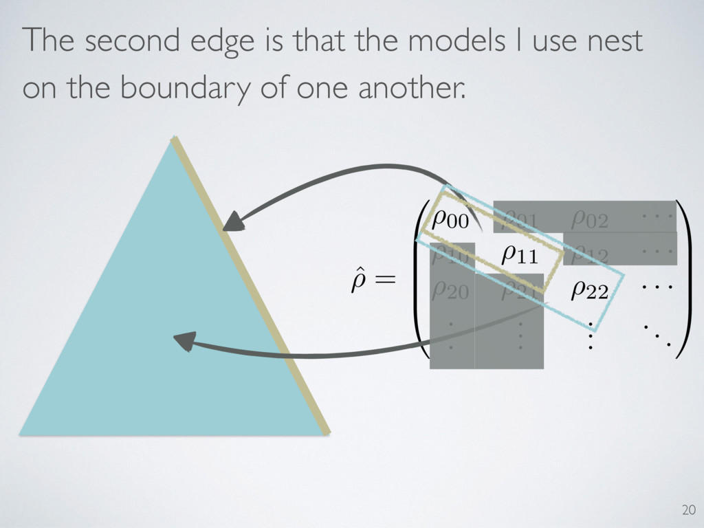
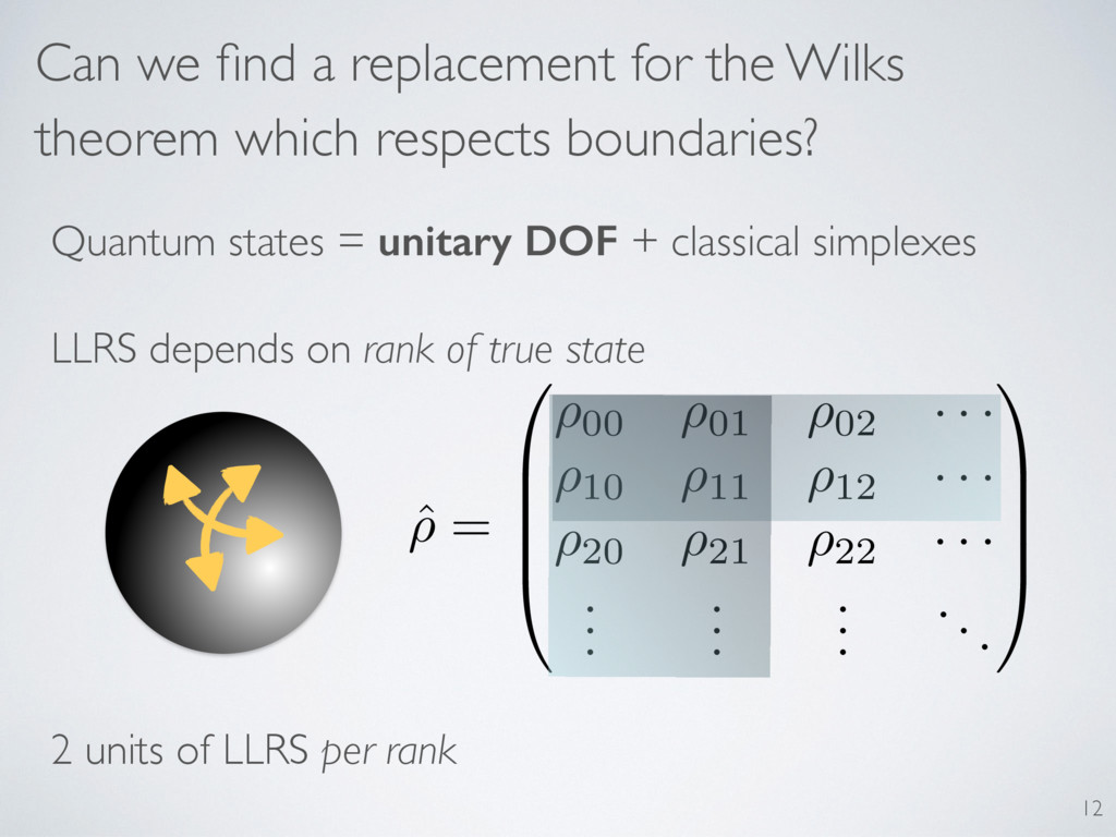
48. Can we find a replacement for the Wilks theorem which respects boundaries? Quantum states = unitary DOF + classical simplexes LLRS depends on rank of true state ˆ ⇢ = 0 B B B @ ⇢00 ⇢01 ⇢02 · · · ⇢10 ⇢11 ⇢12 · · · ⇢20 ⇢21 ⇢22 · · · . . . . . . . . . ... 1 C C C A 2 units of LLRS per rank 12
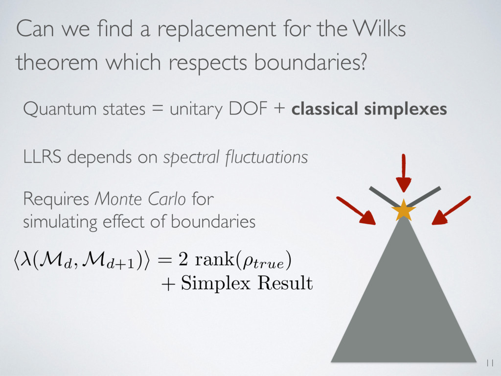
49. Can we find a replacement for the Wilks theorem which respects boundaries? LLRS depends on spectral fluctuations Requires Monte Carlo for
 simulating effect of boundaries Quantum states = unitary DOF + classical simplexes 11 h ( Md, Md+1) i = 2 rank( ⇢true) + Simplex Result
50. How well does this replacement work? Not as accurate as we expected…what is going on? 10
51. How does LLRS behave
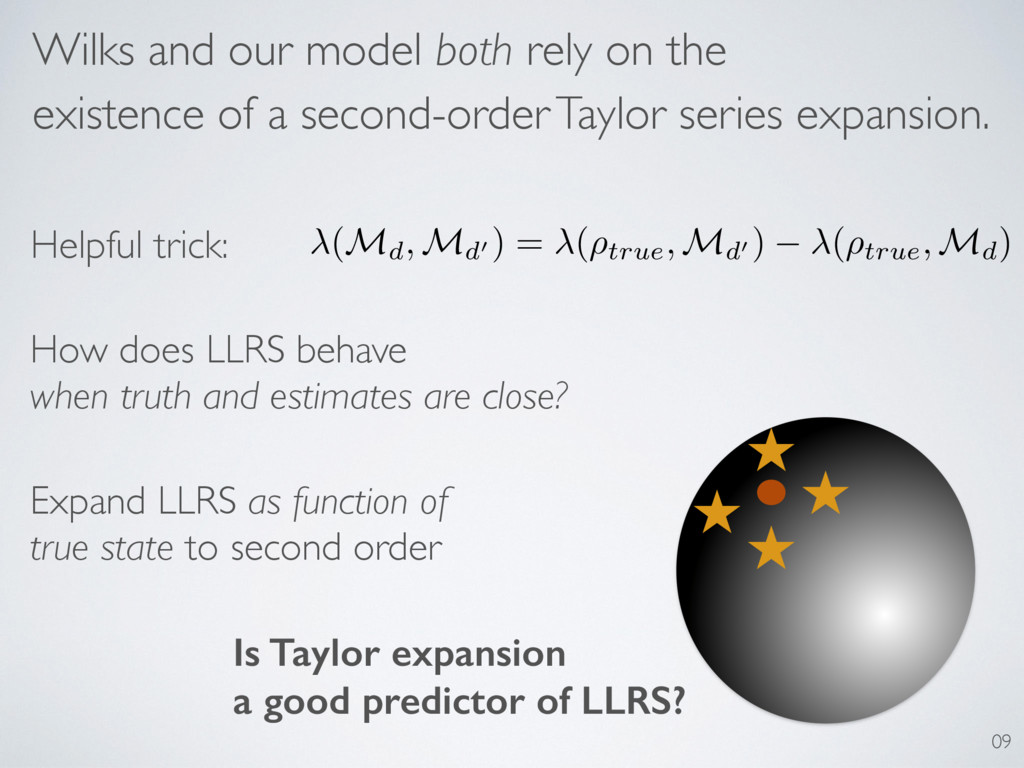
 when truth and estimates are close? Expand LLRS as function of
 true state to second order (Md, Md0 ) = (⇢true, Md0 ) (⇢true, Md) Helpful trick: 09 Wilks and our model both rely on the
 existence of a second-order Taylor series expansion. Is Taylor expansion
 a good predictor of LLRS?
52. Curvature Error Addresses the question “If estimate close to truth,
 what does the LLRS do?” The Taylor series allows us to calculate an approximate expected value. (⇢true, Md) = (⇢true, ˆ ⇢) ⇡ 0 + @ @⇢ ˆ ⇢ (⇢true ˆ ⇢) + 1 2 @2 @⇢2 ˆ ⇢ (⇢true ˆ ⇢)2 h (⇢true, ˆ ⇢)i ⇡ tr ✓⌧ @2L @⇢2 ˆ ⇢ |⇢true ˆ ⇢iihh⇢true ˆ ⇢| ◆ 08
53. In the absence of any boundaries,
 the expected value equals that of Wilks. \ h ( ⇢0, ˆ ⇢ )i ⇡ tr ⇣ ˆ I (ˆ ⇢ ) Cov (ˆ ⇢ ) ⌘ ⇡ d 2 1 No boundaries = no bias in MLE Does not predict distribution, however h (⇢0, ˆ ⇢)i ⇡ tr ✓⌧ @2L @⇢2 ˆ ⇢ |⇢0 ˆ ⇢iihh⇢0 ˆ ⇢| ◆ 07
54. Taylor series seems inaccurate…is something wrong? Most likely. 06 Asymptotic limit? Error in code? We shall see!
55. What was the point of
 all that math?
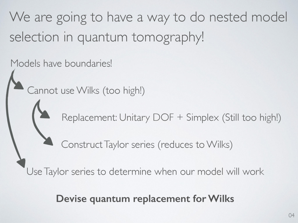
56. We are going to have a way to do nested model selection in quantum tomography! Cannot use Wilks (too high!) Replacement: Unitary DOF + Simplex (Still too high!) 04 Models have boundaries! Construct Taylor series (reduces to Wilks) Use Taylor series to determine when our model will work Devise quantum replacement for Wilks
57. What is next?
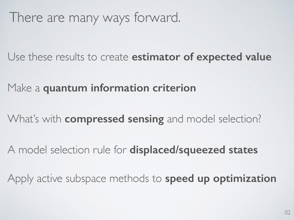
58. There are many ways forward. Use these results to create estimator of expected value Make a quantum information criterion A model selection rule for displaced/squeezed states Apply active subspace methods to speed up optimization What’s with compressed sensing and model selection? 02
59. A year ago, I thought
 model selection using
 the LLRS was easy…
 Today, I am certain it is
 vastly harder than I
 (and others!) thought.
60. Model selection in
 quantum state tomography
 is hard because we
 have to deal with boundaries.