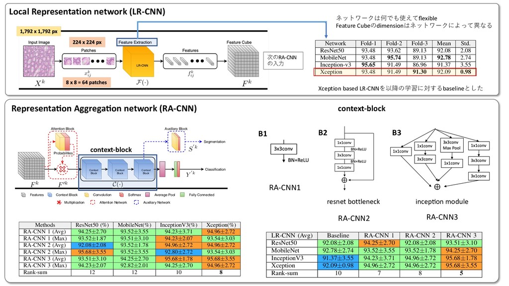
Attention 3に1x1のconv + softmaxを挟んだAttention Blockをさらに追加 1. Standard ベースライン.Lclsを⼩さくするだけ F. Representation Aggregation for Context Learning The local representation tissue has been learned by the LR- CNN. Therefore, the task of spatial context learning from feature-cube is relatively less challenging as compared to context learning from the raw image. A cascaded set of three context blocks (C(·)) of the same type (B1 ,B2 , or B3 ) is used in RA-CNN. These context blocks are explained in section III-E. The output of C(·) is followed by a global average pooling, a fully connected, and a softmax layer to make the final prediction in the required number of classes. The final prediction Y0 from the features of input images X is computed as: Y0 = C(F0, ✓C) ! Lg p (•) ! Lf (•, ✓f0 ) ! Ls(•), (5) where ✓C and ✓f0 represent the parameters of all context blocks and the fully connected layer in RA-CNN, respectively. The proposed framework is trained end-to-end with categorical cross-entropy loss based cost function Lcls(·) which is defined as: Lcls(Y, Y0) = 1 K K X k=1 C X c=1 Y k c log2 (Y 0k c ), (6) where Y k c and Y 0k c are the ground truth and predicted proba- bilities of kth image for cth class. where ↵ is a hyper-parameter which defines the contribution of both loss functions in the final loss. Similar to patch clas- sifier, the loss function (Ljoint ) is minimized with RMSprop optimizer [38]. H. Training Strategies We trained the proposed framework in four different ways with varying ability to capture the spatial context. First, the proposed framework is trained without attention block and by minimizing the Lcls(·) loss only. This configuration is represented by solid line blocks in Fig 2. Second, the same configuration as first but trained with a sample-based weighted loss function, Lwgt(·), which give more weight to the image patches with relatively less region of interest (glandular region) as compared to the background. The weight of an image and Lwgt(·) are defined as follow, Wk = ( 1 Rk roi , if Rk roi > ↵ 1 ↵ , otherwise (10) Lwgt(Y, Y0) = 1 K K X k=1 C X c=1 WkY k c log2 (Y 0k c ), (11) where Rk roi and Wk represent the ratio of the region of interest and weight of the kth image. The ↵ is the ratio threshold, selected empirically as 0.10, sets the upper limit 3. Auxiliary Auxiliary Blockを追加して分類とセグメンテーションの両⽅のロスを計算 where L1⇥1 c and L3⇥3 c denote the convolution layers with 1⇥1 and 3 ⇥ 3 filter sizes; ✓B1 2 , ✓B2 2 , and ✓B3 2 are the parameters of different convolution layers and ✓B2 represents parameter of the whole context block for brevity. The operator represents the concatenation of feature-maps. Unlike the previous two context blocks, our third CB processes the input feature-maps in parallel with different filter sizes to capture context from varying receptive fields. Similar to the blocks in [35], it consists of multiple 1 ⇥ 1 and 3 ⇥ 3 convolution layers each followed by batch normalization and ReLU activation. A 3 ⇥ 3 average pooling layer L3⇥3 p is also used to average the local context information. The CB, B3 , is defined as: B3(F0, ✓B3 ) = [L1⇥1 c (F0, ✓B1 3 ) ! L3⇥3 c (•, ✓B2 3 ) ! L3⇥3 c (•, ✓B3 3 )] [L1⇥1 c (F0, ✓B4 3 )] [L1⇥1 c (F0, ✓B5 3 ) ! L3⇥3 c (•, ✓B6 3 )] [L3⇥3 p (F0) ! L1⇥1 c (•, ✓B7 3 )], (4) where ✓B1 3 to ✓B7 3 are the parameters of different convolution layers and ✓B3 represents parameter of the whole context block for the sake of notational simplicity. F. Representation Aggregation for Context Learning The local representation tissue has been learned by the LR- CNN. Therefore, the task of spatial context learning from feature-cube is relatively less challenging as compared to context learning from the raw image. A cascaded set of three context blocks (C(·)) of the same type (B1 ,B2 , or B3 ) is used in RA-CNN. These context blocks are explained in section III-E. The output of C(·) is followed by a global average pooling, a fully connected, and a softmax layer to make the final prediction in the required number of classes. The final prediction Y0 from the features of input images X is computed primitive structures in the input image. This will improve the convergence of proposed networks and also output the coarse patch based segmentation mask (S0 s ) along with image label (Y 0). The segmentation masks (S0) of input images X from their features F0 is defined as: S0 = C(F0, ✓C) ! L1⇥1 c (•, ✓c0 ) ! Ls(•), (7) where L1⇥1 c is a convolution layer with ✓c0 parameters. The addition of auxiliary block enables the proposes framework to learn in a multi-task setting, where the coarse segmentation- map guides the network to improve the individual patch based feature classification in addition to the prediction of the input image. This leads to a network with improved classifica- tion performance since it is minimizing both segmentation and classification loss simultaneously. The segmentation-map based loss function (Lseg ) and joint loss function (Ljoint ) are defined as: Lseg(S, S0) = 1 K K X k=1 C X c=1 Sk c log2 (S0k c ), (8) Ljoint(Y, Y0, S, S0) =↵ ⇥ Lcls(Y, Y0)+ (1 ↵) ⇥ Lseg(S, S0), (9) where ↵ is a hyper-parameter which defines the contribution of both loss functions in the final loss. Similar to patch clas- sifier, the loss function (Ljoint ) is minimized with RMSprop optimizer [38]. H. Training Strategies We trained the proposed framework in four different ways with varying ability to capture the spatial context. First, the proposed framework is trained without attention block and by minimizing the Lcls(·) loss only. This configuration is 7 xity. The performance of these classifiers for CRC g is reported in Table III. Although, the performance classifiers is comparable, MobileNet shows superior mance with highest mean accuracy. On the other hand, on classifier shows consistent performance across three with the lowest standard deviation (Std.). TABLE III ACCURACY COMPARISON OF FOUR PATCH CLASSIFIERS. Network Fold-1 Fold-2 Fold-3 Mean Std. ResNet50 93.48 93.62 89.13 92.08 2.08 MobileNet 93.48 95.74 89.13 92.78 2.74 nception-v3 95.65 91.49 86.96 91.37 3.55 Xception 93.48 91.49 91.30 92.09 0.98 TABLE V ROBUSTNESS ANALYSIS OF FEATURE EXTRACTORS ACROSS DIFFERENT METHODS. Methods ResNet50 (%) MobileNet(%) InceptionV3(%) Xception(%) RA-CNN 1 (Avg) 94.25±2.70 93.52±3.55 94.23±3.71 94.96±2.72 RA-CNN 1 (Max) 93.52±1.87 93.51±3.10 94.23±2.07 93.54±3.03 RA-CNN 2 (Avg) 92.08±2.08 93.52±1.78 94.96±2.72 94.96±2.72 RA-CNN 2 (Max) 95.68±3.55 93.52±3.55 92.80±2.72 93.54±3.03 RA-CNN 3 (Avg) 93.51±3.10 94.25±2.70 95.68±1.78 95.68±3.55 RA-CNN 3 (Max) 94.23±2.07 92.82±2.01 94.25±2.70 94.96±2.72 Rank-sum 12 12 10 8 TABLE VI COMPARISON FOR DIFFERENT TRAINING STRATEGIES WITH XCEPTION AS FEATURE EXTRACTOR. Feature Standard Weighted Auxiliary Attention Xception - Max 94.01 94.49 94.73 95.21 Xception - Avg 95.20 94.72 94.72 94.00 Mean 94.61 94.60 94.72 94.61 3 LR-CNN RA-CNN 4 er L3⇥3 p is also The CB, B3 , is •, ✓B2 3 ) F0, ✓B4 3 )] •, ✓B6 3 )] 7 3 )], (4) ent convolution e context block rning ned by the LR- learning from compared to ed set of three or B3 ) is used ned in section global average er to make the sses. The final X is computed ! Ls(•), (5) context blocks spectively. The ith categorical hich is defined Y 0k c ), (6) learn in a multi-task setting, where the coarse segmentation- map guides the network to improve the individual patch based feature classification in addition to the prediction of the input image. This leads to a network with improved classifica- tion performance since it is minimizing both segmentation and classification loss simultaneously. The segmentation-map based loss function (Lseg ) and joint loss function (Ljoint ) are defined as: Lseg(S, S0) = 1 K K X k=1 C X c=1 Sk c log2 (S0k c ), (8) Ljoint(Y, Y0, S, S0) =↵ ⇥ Lcls(Y, Y0)+ (1 ↵) ⇥ Lseg(S, S0), (9) where ↵ is a hyper-parameter which defines the contribution of both loss functions in the final loss. Similar to patch clas- sifier, the loss function (Ljoint ) is minimized with RMSprop optimizer [38]. H. Training Strategies We trained the proposed framework in four different ways with varying ability to capture the spatial context. First, the proposed framework is trained without attention block and by minimizing the Lcls(·) loss only. This configuration is represented by solid line blocks in Fig 2. Second, the same configuration as first but trained with a sample-based weighted loss function, Lwgt(·), which give more weight to the image patches with relatively less region of interest (glandular region) as compared to the background. The weight of an image and Lwgt(·) are defined as follow, Wk = ( 1 Rk roi , if Rk roi > ↵ 1 ↵ , otherwise (10) Lwgt(Y, Y0) = 1 K K X k=1 C X c=1 WkY k c log2 (Y 0k c ), (11) α=0.1 A. Network Input The input to our framework is an image (Xk) from a dataset, D = {Xk, Y k, Sk; k = 1, . . . K}, of large high resolution images which consists of K images with corresponding labels Y k 2 {1, . . . , C} for classification into C classes and coarse patch level segmentation masks Sk 2 {1, . . . , C} for multi- task learning. Each image is divided into M ⇥ N patches of same size where xk ij and yk ij represent the ijth patch of kth image and its corresponding label, respectively. We used a patch dataset, d = {(xk ij , yk ij ), | xk ij 2 Xk, yk ij 2 Y k}, which consists of patches and their corresponding labels for pre- training of LR-CNN. B. Local Representation Learning First part of the proposed framework encodes an input image Xk into a feature-cube Fk. All the input images are processed through the LR-CNN in a patch based manner. The proposed framework is flexible enough to use any state-of- the-art image classifier as a LR-CNN such as ResNet50 [33], MobileNet [34], Inception [35], or Xception [36]. This flex- ibility also enables it to use pre-trained weights in case of a limited dataset. Moreover, it is possible to train the LR-CNN independently before plugging it into the proposed framework, enabling it to learn meaningful representation [37] which leads to early convergence of the context-aware learning part of the framework. each value in the feature-cube. Hadamard product is taken between the weights and input feature-cube to increase the impact of more important areas of an image in label prediction and vice-versa. The weighted feature-cube F0 is defined as: F0 = L1⇥1 c (F, ✓c) ! Ls(•) ⌦ F, (2) where L1⇥1 c and ✓c represent the 1 ⇥ 1 convolution layer and its parameters, respectively. Ls denotes the softmax layer and the operator ⌦ is used to represent Hadamard product. E. Context Blocks Since the LR-CNN is used to encode the important patch- based image representation into a feature-cube, therefore the main aim of the context block (CB) is to learn the spatial context within the feature cube. The CB learns the relation between the features of the image patches considering their spatial location. We propose three different CB architectures, each with different complexity and capability to capture the context information. First CB, B1(·), is comprised of a 3 ⇥ 3 convolution layer followed by ReLU activation and batch normalization. Second CB, B2(·), uses residual block [33] architecture with two different filter sizes. It consists of three convolution layers each followed by batch normalization and ReLU activation. The first and last layers are with 1 ⇥ 1 convolution filter to squeeze and expand the feature depth. The ! L3⇥3 c (•, ✓B3 3 )] [L1⇥1 c (F0, ✓B4 3 )] [L1⇥1 c (F0, ✓B5 3 ) ! L3⇥3 c (•, ✓B6 3 )] [L3⇥3 p (F0) ! L1⇥1 c (•, ✓B7 3 )], (4) where ✓B1 3 to ✓B7 3 are the parameters of different convolution layers and ✓B3 represents parameter of the whole context block for the sake of notational simplicity. F. Representation Aggregation for Context Learning The local representation tissue has been learned by the LR- CNN. Therefore, the task of spatial context learning from feature-cube is relatively less challenging as compared to context learning from the raw image. A cascaded set of three context blocks (C(·)) of the same type (B1 ,B2 , or B3 ) is used in RA-CNN. These context blocks are explained in section III-E. The output of C(·) is followed by a global average pooling, a fully connected, and a softmax layer to make the final prediction in the required number of classes. The final prediction Y0 from the features of input images X is computed as: Y0 = C(F0, ✓C) ! Lg p (•) ! Lf (•, ✓f0 ) ! Ls(•), (5) where ✓C and ✓f0 represent the parameters of all context blocks and the fully connected layer in RA-CNN, respectively. The proposed framework is trained end-to-end with categorical cross-entropy loss based cost function Lcls(·) which is defined as: Lcls(Y, Y0) = 1 K K X k=1 C X c=1 Y k c log2 (Y 0k c ), (6) where Y k c and Y 0k c are the ground truth and predicted proba- bilities of kth image for cth class. and classification loss simultaneously. The segmentation based loss function (Lseg ) and joint loss function (Ljoint defined as: Lseg(S, S0) = 1 K K X k=1 C X c=1 Sk c log2 (S0k c ), Ljoint(Y, Y0, S, S0) =↵ ⇥ Lcls(Y, Y0)+ (1 ↵) ⇥ Lseg(S, S0), where ↵ is a hyper-parameter which defines the contrib of both loss functions in the final loss. Similar to patch sifier, the loss function (Ljoint ) is minimized with RMS optimizer [38]. H. Training Strategies We trained the proposed framework in four different with varying ability to capture the spatial context. First proposed framework is trained without attention block by minimizing the Lcls(·) loss only. This configuratio represented by solid line blocks in Fig 2. Second, the configuration as first but trained with a sample-based weig loss function, Lwgt(·), which give more weight to the im patches with relatively less region of interest (glandular reg as compared to the background. The weight of an image Lwgt(·) are defined as follow, Wk = ( 1 Rk roi , if Rk roi > ↵ 1 ↵ , otherwise Lwgt(Y, Y0) = 1 K K X k=1 C X c=1 WkY k c log2 (Y 0k c ), where Rk roi and Wk represent the ratio of the regio interest and weight of the kth image. The ↵ is the threshold, selected empirically as 0.10, sets the upper Xception RA-CNN3