Introduction to Data Analysis and Visualization using R

Outline Introduction Data Structures Working with Data Visualisation Webapps Integration
with other Systems Data Analysis and Visualisation using R Vinayak Hegde July 11, 2013 1 / 124

with other Systems Outline of Topics I 1 Introduction About R Workspace Basics Basic functions Basic Statistics functions Basic Plotting Functions Basic library functions Resources 2 Data Structures Vector Matrix Array 2 / 124

with other Systems Outline of Topics II Data Frames Factors List Basic datastucture functions 3 Working with Data Reading Data Transforming Data Live example 4 Visualisation Introduction Basic plots Advanced Plots 3 / 124

with other Systems Outline of Topics III Grammar of Graphics 5 Webapps Introduction to Shiny Features Architecture Code example 6 Integration with other Systems 4 / 124

with other Systems About R Workspace Basics Basic functions Basic Statistics functions Basic Plotting Functions Basic library functions Resources Outline 1 Introduction 2 Data Structures 3 Working with Data 4 Visualisation 5 Webapps 6 Integration with other Systems 5 / 124

with other Systems About R Workspace Basics Basic functions Basic Statistics functions Basic Plotting Functions Basic library functions Resources What is R ? Wikipedia R is a free software programming language and a software environment for statistical computing and graphics. The R language is widely used among statisticians and data miners for developing statistical software and data analysis. 6 / 124

with other Systems About R Workspace Basics Basic functions Basic Statistics functions Basic Plotting Functions Basic library functions Resources Why use R ? Designed and optimised for data processing Lots of modules State of the art graphics Free as in freedom/beer Helpful community Very ﬂexible and good integration 7 / 124

with other Systems About R Workspace Basics Basic functions Basic Statistics functions Basic Plotting Functions Basic library functions Resources R Studio Installation Go to RStudio website Download the server/desktop version For server - Open the browser and go to http://127.0.0.1:8787 For desktop - Click on the shortcut and you are ready to go 8 / 124

with other Systems About R Workspace Basics Basic functions Basic Statistics functions Basic Plotting Functions Basic library functions Resources R Studio Basics The Source Editor The Console / Interpreter Workspace / History Plots / Packages / Help 9 / 124

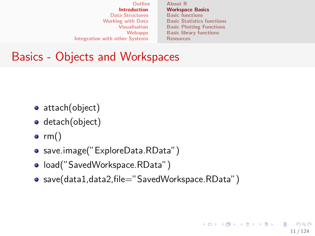
with other Systems About R Workspace Basics Basic functions Basic Statistics functions Basic Plotting Functions Basic library functions Resources Basics - Starting oﬀ and getting help Starting the interpreter Getting online help - ? or help() Searching for help - ?? Approximate search - apropos() 10 / 124

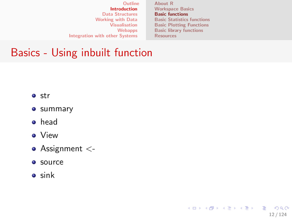
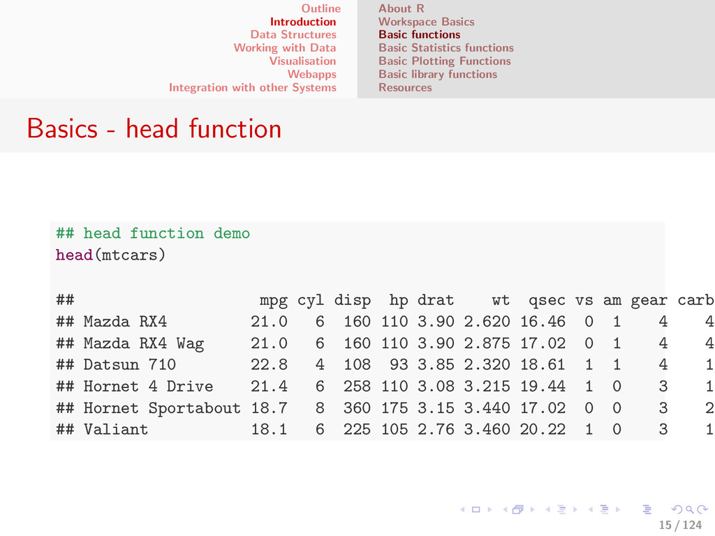
with other Systems About R Workspace Basics Basic functions Basic Statistics functions Basic Plotting Functions Basic library functions Resources Basics - Objects and Workspaces attach(object) detach(object) rm() save.image(”ExploreData.RData”) load(”SavedWorkspace.RData”) save(data1,data2,ﬁle=”SavedWorkspace.RData”) 11 / 124

with other Systems About R Workspace Basics Basic functions Basic Statistics functions Basic Plotting Functions Basic library functions Resources Basics - Using inbuilt function str summary head View Assignment <- source sink 12 / 124

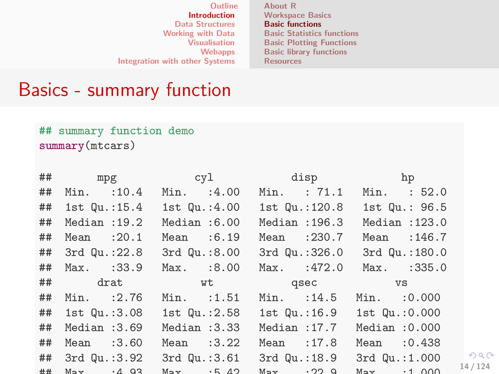
with other Systems About R Workspace Basics Basic functions Basic Statistics functions Basic Plotting Functions Basic library functions Resources Basics - str function ## str function demo str(mtcars) ## 'data.frame': 32 obs. of 11 variables: ## $ mpg : num 21 21 22.8 21.4 18.7 18.1 14.3 24.4 22.8 19.2 ... ## $ cyl : num 6 6 4 6 8 6 8 4 4 6 ... ## $ disp: num 160 160 108 258 360 ... ## $ hp : num 110 110 93 110 175 105 245 62 95 123 ... ## $ drat: num 3.9 3.9 3.85 3.08 3.15 2.76 3.21 3.69 3.92 3.92 ... ## $ wt : num 2.62 2.88 2.32 3.21 3.44 ... ## $ qsec: num 16.5 17 18.6 19.4 17 ... ## $ vs : num 0 0 1 1 0 1 0 1 1 1 ... ## $ am : num 1 1 1 0 0 0 0 0 0 0 ... ## $ gear: num 4 4 4 3 3 3 3 4 4 4 ... ## $ carb: num 4 4 1 1 2 1 4 2 2 4 ... 13 / 124

with other Systems About R Workspace Basics Basic functions Basic Statistics functions Basic Plotting Functions Basic library functions Resources Basics - summary function ## summary function demo summary(mtcars) ## mpg cyl disp hp ## Min. :10.4 Min. :4.00 Min. : 71.1 Min. : 52.0 ## 1st Qu.:15.4 1st Qu.:4.00 1st Qu.:120.8 1st Qu.: 96.5 ## Median :19.2 Median :6.00 Median :196.3 Median :123.0 ## Mean :20.1 Mean :6.19 Mean :230.7 Mean :146.7 ## 3rd Qu.:22.8 3rd Qu.:8.00 3rd Qu.:326.0 3rd Qu.:180.0 ## Max. :33.9 Max. :8.00 Max. :472.0 Max. :335.0 ## drat wt qsec vs ## Min. :2.76 Min. :1.51 Min. :14.5 Min. :0.000 ## 1st Qu.:3.08 1st Qu.:2.58 1st Qu.:16.9 1st Qu.:0.000 ## Median :3.69 Median :3.33 Median :17.7 Median :0.000 ## Mean :3.60 Mean :3.22 Mean :17.8 Mean :0.438 ## 3rd Qu.:3.92 3rd Qu.:3.61 3rd Qu.:18.9 3rd Qu.:1.000 14 / 124

with other Systems About R Workspace Basics Basic functions Basic Statistics functions Basic Plotting Functions Basic library functions Resources Basics - head function ## head function demo head(mtcars) ## mpg cyl disp hp drat wt qsec vs am gear carb ## Mazda RX4 21.0 6 160 110 3.90 2.620 16.46 0 1 4 4 ## Mazda RX4 Wag 21.0 6 160 110 3.90 2.875 17.02 0 1 4 4 ## Datsun 710 22.8 4 108 93 3.85 2.320 18.61 1 1 4 1 ## Hornet 4 Drive 21.4 6 258 110 3.08 3.215 19.44 1 0 3 1 ## Hornet Sportabout 18.7 8 360 175 3.15 3.440 17.02 0 0 3 2 ## Valiant 18.1 6 225 105 2.76 3.460 20.22 1 0 3 1 15 / 124

with other Systems About R Workspace Basics Basic functions Basic Statistics functions Basic Plotting Functions Basic library functions Resources Basics - Inbuilt Statistics functions mean sd var median quantile hist plot 16 / 124

with other Systems About R Workspace Basics Basic functions Basic Statistics functions Basic Plotting Functions Basic library functions Resources Basics - Stats Functions Demo set.seed(1729) x = rnorm(25) mean(x) ## [1] 0.1951 var(x) ## [1] 0.5624 sd(x) ## [1] 0.7499 17 / 124

with other Systems About R Workspace Basics Basic functions Basic Statistics functions Basic Plotting Functions Basic library functions Resources Basics - Stats Functions Demo median(x) ## [1] 0.08827 quantile(x) ## 0% 25% 50% 75% 100% ## -1.40843 -0.31371 0.08827 0.52097 1.96241 18 / 124

with other Systems About R Workspace Basics Basic functions Basic Statistics functions Basic Plotting Functions Basic library functions Resources Basics - Stats Functions Demo hist(x) plot(x) Histogram of x x Frequency −1.5 −1.0 −0.5 0.0 0.5 1.0 1.5 2.0 0 2 4 6 8 5 10 15 20 25 −1.5 −0.5 0.0 0.5 1.0 1.5 2.0 Index x 19 / 124

with other Systems About R Workspace Basics Basic functions Basic Statistics functions Basic Plotting Functions Basic library functions Resources Basics - Library commands install.packages(”packagename”) library(”package”) update.packages(”packages”) search() detach(”package:packagename”) 20 / 124

with other Systems About R Workspace Basics Basic functions Basic Statistics functions Basic Plotting Functions Basic library functions Resources Install Views install.views(”packageGroupName”) update.views(”packageGroupName”) Package Groups Econometrics Graphics TimeSeries HighPerformanceComputing Optimization 21 / 124

with other Systems About R Workspace Basics Basic functions Basic Statistics functions Basic Plotting Functions Basic library functions Resources Resources R Project R Seek R Documentation R Journal CRAN 22 / 124

with other Systems Vector Matrix Array Data Frames Factors List Basic datastucture functions Outline 1 Introduction 2 Data Structures 3 Working with Data 4 Visualisation 5 Webapps 6 Integration with other Systems 23 / 124

with other Systems Vector Matrix Array Data Frames Factors List Basic datastucture functions Vector Vector Datastructure Vectors are one-dimensional arrays that can hold numeric data, character data, or logical data. Vectors can be column vectors (created with c()) or row vectors(can be created using the transpose function t()). 24 / 124

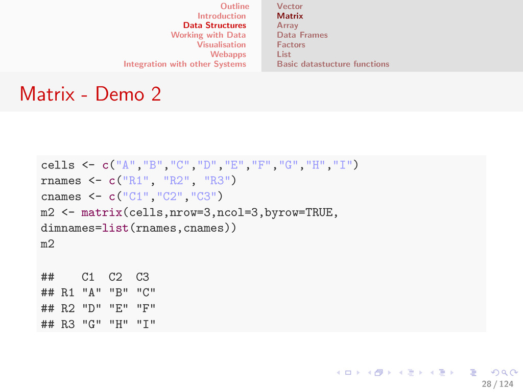
with other Systems Vector Matrix Array Data Frames Factors List Basic datastucture functions Vector - Demo a <- c(1, 4, 3, -1, 0, 2, 9) b <- c("Apples", "Oranges", "Banana", "Mango") c <- c(FALSE, TRUE, TRUE, FALSE) a[4] ## [1] -1 b[c(2, 4)] ## [1] "Oranges" "Mango" c[2:4] ## [1] TRUE TRUE FALSE 25 / 124

with other Systems Vector Matrix Array Data Frames Factors List Basic datastucture functions Matrix Matrix Datastructure A matrix is a two-dimensional array where each element has the same mode (numeric, character, or logical). Matrices are created with the matrix() function. 26 / 124

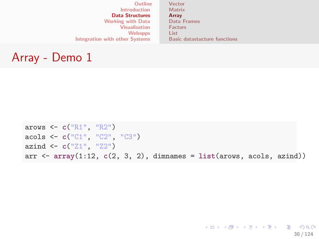
with other Systems Vector Matrix Array Data Frames Factors List Basic datastucture functions Matrix - Demo 1 m1 <- matrix(1:20, nrow = 5, ncol = 4) m1 ## [,1] [,2] [,3] [,4] ## [1,] 1 6 11 16 ## [2,] 2 7 12 17 ## [3,] 3 8 13 18 ## [4,] 4 9 14 19 ## [5,] 5 10 15 20 27 / 124

with other Systems Vector Matrix Array Data Frames Factors List Basic datastucture functions Matrix - Demo 2 cells <- c("A","B","C","D","E","F","G","H","I") rnames <- c("R1", "R2", "R3") cnames <- c("C1","C2","C3") m2 <- matrix(cells,nrow=3,ncol=3,byrow=TRUE, dimnames=list(rnames,cnames)) m2 ## C1 C2 C3 ## R1 "A" "B" "C" ## R2 "D" "E" "F" ## R3 "G" "H" "I" 28 / 124

with other Systems Vector Matrix Array Data Frames Factors List Basic datastucture functions Array Array Datastructure Arrays are similar to matrices but can have more than two dimensions. Theyre created with an array() function. Like matrices, they can contain only one datatype. 29 / 124

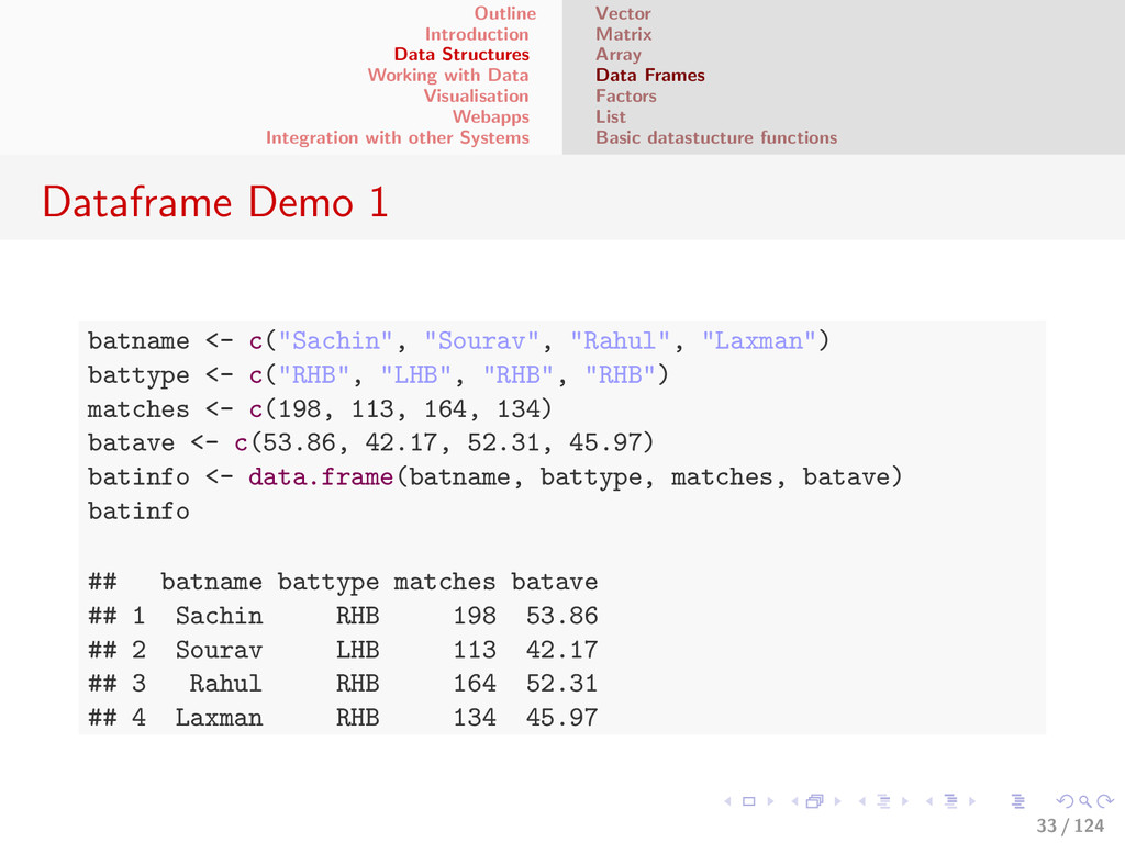
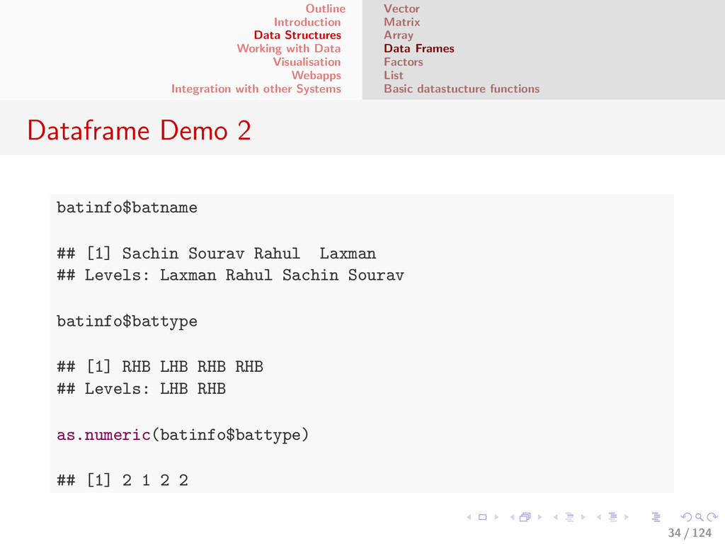
with other Systems Vector Matrix Array Data Frames Factors List Basic datastucture functions Array - Demo 1 arows <- c("R1", "R2") acols <- c("C1", "C2", "C3") azind <- c("Z1", "Z2") arr <- array(1:12, c(2, 3, 2), dimnames = list(arows, acols, azind)) 30 / 124

with other Systems Vector Matrix Array Data Frames Factors List Basic datastucture functions Array - Demo 2 arr ## , , Z1 ## ## C1 C2 C3 ## R1 1 3 5 ## R2 2 4 6 ## ## , , Z2 ## ## C1 C2 C3 ## R1 7 9 11 ## R2 8 10 12 31 / 124

with other Systems Vector Matrix Array Data Frames Factors List Basic datastucture functions Data Frames Data Frame Datastructure A Dataframe is like a matrix but each of the columns can be a diﬀerent datatype. Another way to think about it is as a bunch of diﬀerent types of columns with similar keys (like a database table). A dataframe is created with the data.frame() function. 32 / 124

with other Systems Vector Matrix Array Data Frames Factors List Basic datastucture functions Dataframe Demo 1 batname <- c("Sachin", "Sourav", "Rahul", "Laxman") battype <- c("RHB", "LHB", "RHB", "RHB") matches <- c(198, 113, 164, 134) batave <- c(53.86, 42.17, 52.31, 45.97) batinfo <- data.frame(batname, battype, matches, batave) batinfo ## batname battype matches batave ## 1 Sachin RHB 198 53.86 ## 2 Sourav LHB 113 42.17 ## 3 Rahul RHB 164 52.31 ## 4 Laxman RHB 134 45.97 33 / 124

with other Systems Vector Matrix Array Data Frames Factors List Basic datastucture functions Dataframe Demo 2 batinfo$batname ## [1] Sachin Sourav Rahul Laxman ## Levels: Laxman Rahul Sachin Sourav batinfo$battype ## [1] RHB LHB RHB RHB ## Levels: LHB RHB as.numeric(batinfo$battype) ## [1] 2 1 2 2 34 / 124

with other Systems Vector Matrix Array Data Frames Factors List Basic datastucture functions Dataframe Demo 3 summary(batinfo) ## batname battype matches batave ## Laxman:1 LHB:1 Min. :113 Min. :42.2 ## Rahul :1 RHB:3 1st Qu.:129 1st Qu.:45.0 ## Sachin:1 Median :149 Median :49.1 ## Sourav:1 Mean :152 Mean :48.6 ## 3rd Qu.:172 3rd Qu.:52.7 ## Max. :198 Max. :53.9 35 / 124

with other Systems Vector Matrix Array Data Frames Factors List Basic datastucture functions Factors Factors are made of categorical data Factors can be ordered or unordered Factors are represented internally as numbers Assignment is by alphabetical order 36 / 124

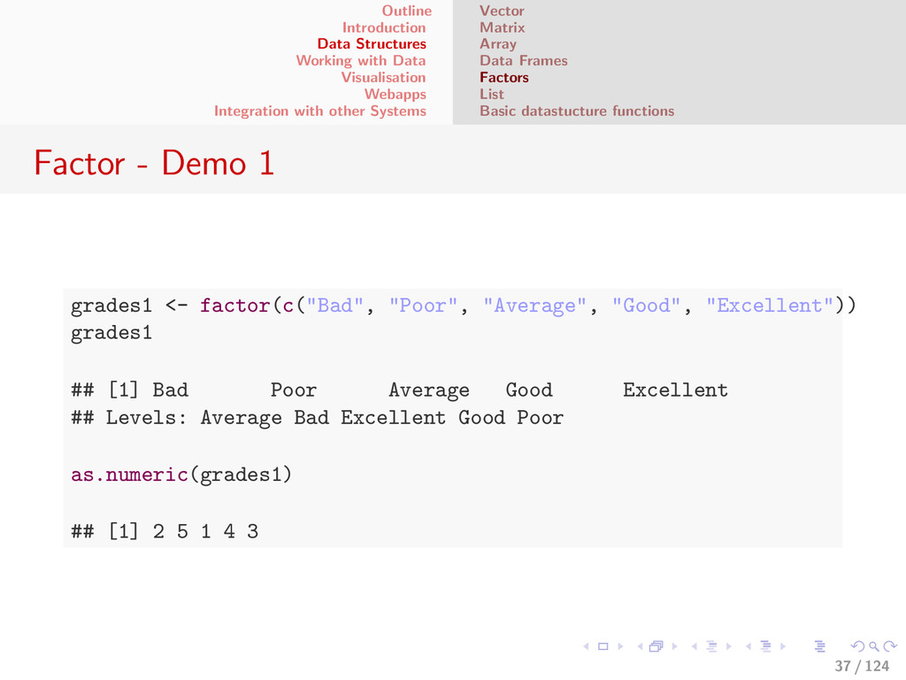
with other Systems Vector Matrix Array Data Frames Factors List Basic datastucture functions Factor - Demo 1 grades1 <- factor(c("Bad", "Poor", "Average", "Good", "Excellent")) grades1 ## [1] Bad Poor Average Good Excellent ## Levels: Average Bad Excellent Good Poor as.numeric(grades1) ## [1] 2 5 1 4 3 37 / 124

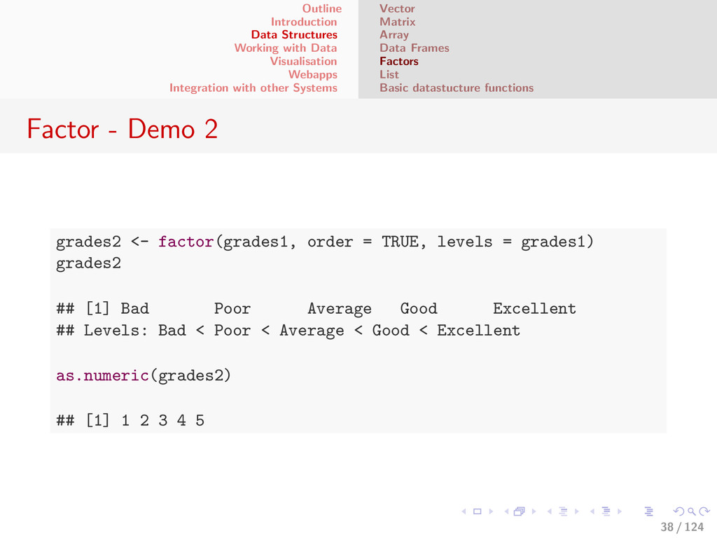
with other Systems Vector Matrix Array Data Frames Factors List Basic datastucture functions Factor - Demo 2 grades2 <- factor(grades1, order = TRUE, levels = grades1) grades2 ## [1] Bad Poor Average Good Excellent ## Levels: Bad < Poor < Average < Good < Excellent as.numeric(grades2) ## [1] 1 2 3 4 5 38 / 124

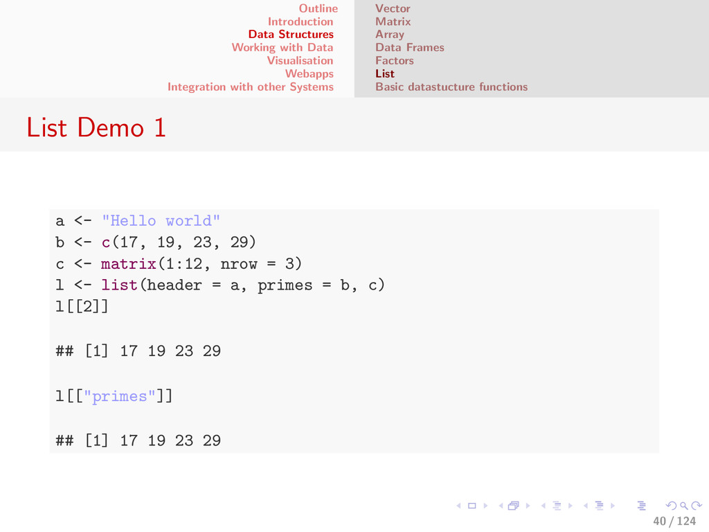
with other Systems Vector Matrix Array Data Frames Factors List Basic datastucture functions List List Datastructure List is a bit of a mixed bag. A list is an ordered collection of objects. A list allows you to gather a variety of (possibly unrelated) objects under one name. A list may contain an arbitrary combination of vectors, matrices, data frames, and even other lists. You create a list using the list() function. 39 / 124

with other Systems Vector Matrix Array Data Frames Factors List Basic datastucture functions List Demo 1 a <- "Hello world" b <- c(17, 19, 23, 29) c <- matrix(1:12, nrow = 3) l <- list(header = a, primes = b, c) l[[2]] ## [1] 17 19 23 29 l[["primes"]] ## [1] 17 19 23 29 40 / 124

with other Systems Vector Matrix Array Data Frames Factors List Basic datastucture functions List Demo 2 l ## $header ## [1] "Hello world" ## ## $primes ## [1] 17 19 23 29 ## ## [[3]] ## [,1] [,2] [,3] [,4] ## [1,] 1 4 7 10 ## [2,] 2 5 8 11 ## [3,] 3 6 9 12 41 / 124

with other Systems Vector Matrix Array Data Frames Factors List Basic datastucture functions Working with Data Structures concatenate c() cbind() rbind() data.frame() mode() class() 42 / 124

with other Systems Vector Matrix Array Data Frames Factors List Basic datastucture functions Working with Data Structures with() sort() subset() select() transform() 43 / 124

with other Systems Vector Matrix Array Data Frames Factors List Basic datastucture functions Working with Data Structures names() row.names() attributes() 44 / 124

with other Systems Reading Data Transforming Data Live example Outline 1 Introduction 2 Data Structures 3 Working with Data 4 Visualisation 5 Webapps 6 Integration with other Systems 45 / 124

with other Systems Reading Data Transforming Data Live example Reading data from multiple Sources Excel ﬁles web pages csv databases 46 / 124

with other Systems Reading Data Transforming Data Live example Reading data in Excel ﬁles library(gdata) read.xls("~/hacknight/All_India_Index_April3.xls", sheet = 1) 47 / 124

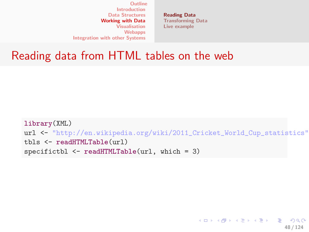
with other Systems Reading Data Transforming Data Live example Reading data from HTML tables on the web library(XML) url <- "http://en.wikipedia.org/wiki/2011_Cricket_World_Cup_statistics" tbls <- readHTMLTable(url) specifictbl <- readHTMLTable(url, which = 3) 48 / 124

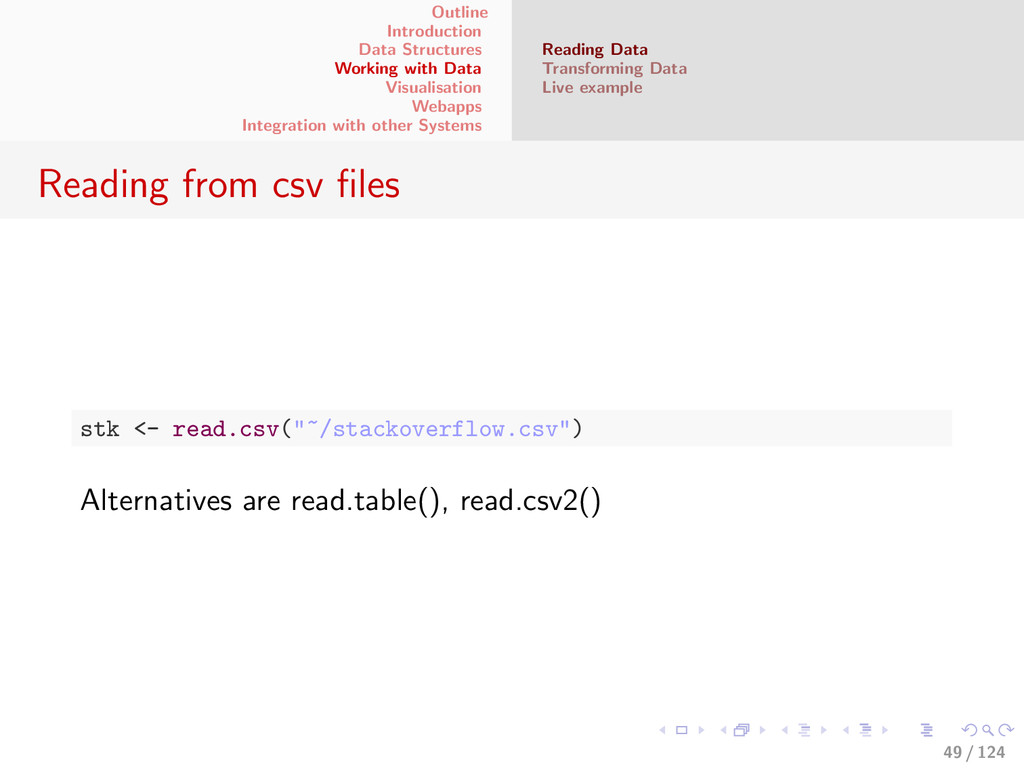
with other Systems Reading Data Transforming Data Live example Reading from csv ﬁles stk <- read.csv("~/stackoverflow.csv") Alternatives are read.table(), read.csv2() 49 / 124

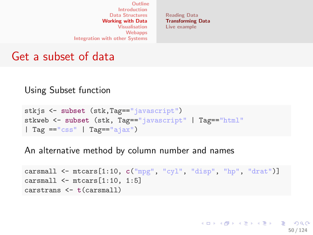
with other Systems Reading Data Transforming Data Live example Get a subset of data Using Subset function stkjs <- subset (stk,Tag=="javascript") stkweb <- subset (stk, Tag=="javascript" | Tag=="html" | Tag =="css" | Tag=="ajax") An alternative method by column number and names carsmall <- mtcars[1:10, c("mpg", "cyl", "disp", "hp", "drat")] carsmall <- mtcars[1:10, 1:5] carstrans <- t(carsmall) 50 / 124

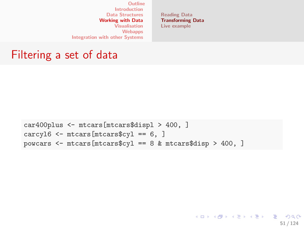
with other Systems Reading Data Transforming Data Live example Filtering a set of data car400plus <- mtcars[mtcars$displ > 400, ] carcyl6 <- mtcars[mtcars$cyl == 6, ] powcars <- mtcars[mtcars$cyl == 8 & mtcars$disp > 400, ] 51 / 124

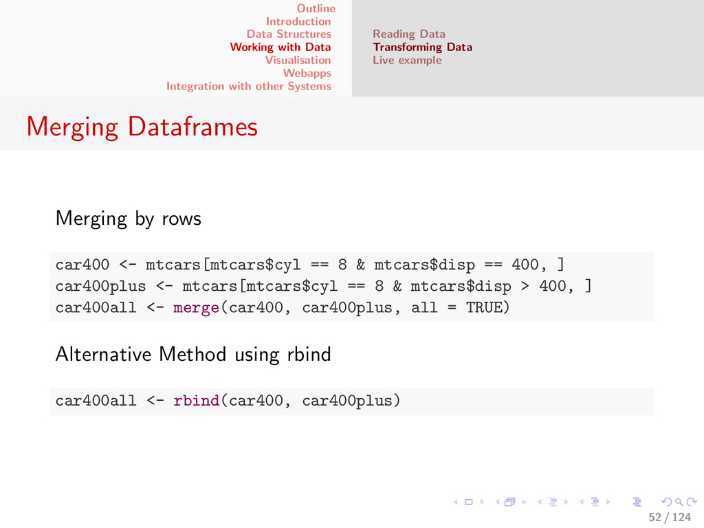
with other Systems Reading Data Transforming Data Live example Merging Dataframes Merging by rows car400 <- mtcars[mtcars$cyl == 8 & mtcars$disp == 400, ] car400plus <- mtcars[mtcars$cyl == 8 & mtcars$disp > 400, ] car400all <- merge(car400, car400plus, all = TRUE) Alternative Method using rbind car400all <- rbind(car400, car400plus) 52 / 124

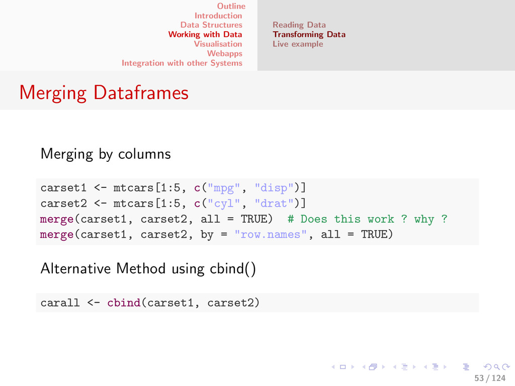
with other Systems Reading Data Transforming Data Live example Merging Dataframes Merging by columns carset1 <- mtcars[1:5, c("mpg", "disp")] carset2 <- mtcars[1:5, c("cyl", "drat")] merge(carset1, carset2, all = TRUE) # Does this work ? why ? merge(carset1, carset2, by = "row.names", all = TRUE) Alternative Method using cbind() carall <- cbind(carset1, carset2) 53 / 124

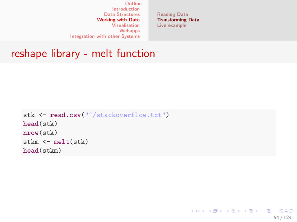
with other Systems Reading Data Transforming Data Live example reshape library - melt function stk <- read.csv("~/stackoverflow.txt") head(stk) nrow(stk) stkm <- melt(stk) head(stkm) 54 / 124

with other Systems Reading Data Transforming Data Live example reshape library - cast function head(stkm) stkm$variable <- as.numeric(sub("X","",stkm$variable)) head(stkm) names(stkm)[2] <- "YearMonth" head(stkm) stkc <- cast(stkm, Tag ~ YearMonth) head(stkc) 55 / 124

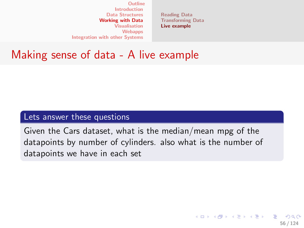
with other Systems Reading Data Transforming Data Live example Making sense of data - A live example Lets answer these questions Given the Cars dataset, what is the median/mean mpg of the datapoints by number of cylinders. also what is the number of datapoints we have in each set 56 / 124

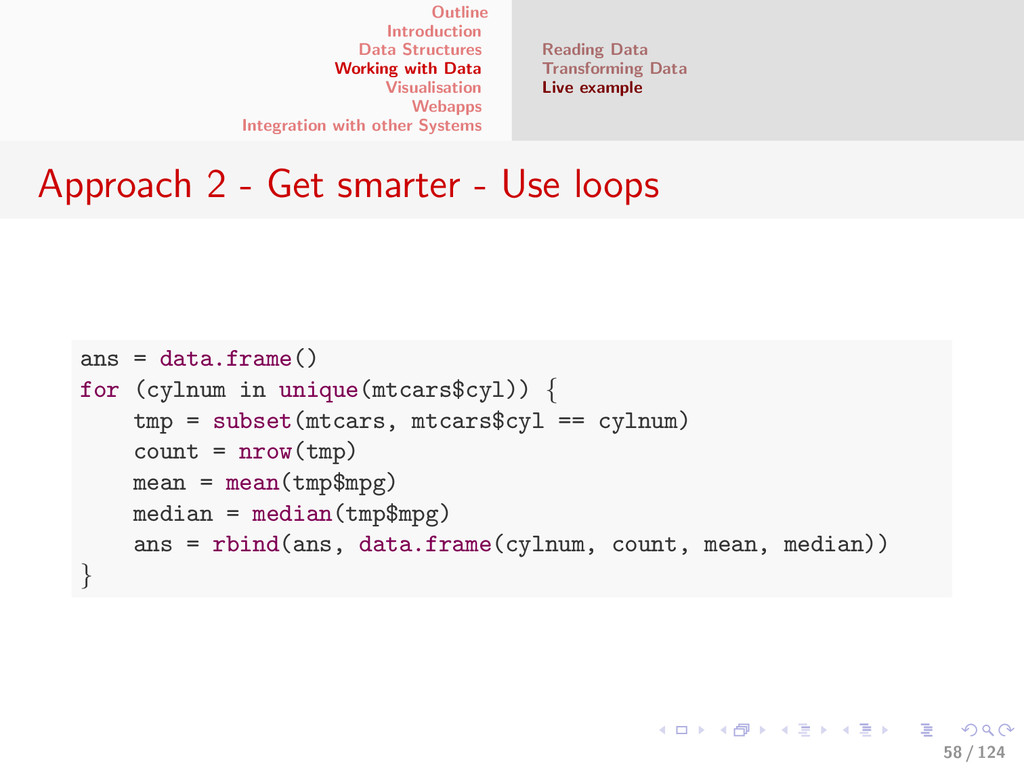
with other Systems Reading Data Transforming Data Live example Approach 1 - Manual approach - Subset and functions unique(mtcars$cyl) cyl4 <- subset(mtcars, cyl == 4) cyl6 <- subset(mtcars, cyl == 6) cyl8 <- subset(mtcars, cyl == 8) nrow(cyl4) nrow(cyl6) nrow(cyl8) mean(cyl6$mpg) mean(cyl4$mpg) mean(cyl8$mpg) median(cyl4$mpg) median(cyl6$mpg) median(cyl8$mpg) 57 / 124

with other Systems Reading Data Transforming Data Live example Approach 2 - Get smarter - Use loops ans = data.frame() for (cylnum in unique(mtcars$cyl)) { tmp = subset(mtcars, mtcars$cyl == cylnum) count = nrow(tmp) mean = mean(tmp$mpg) median = median(tmp$mpg) ans = rbind(ans, data.frame(cylnum, count, mean, median)) } 58 / 124

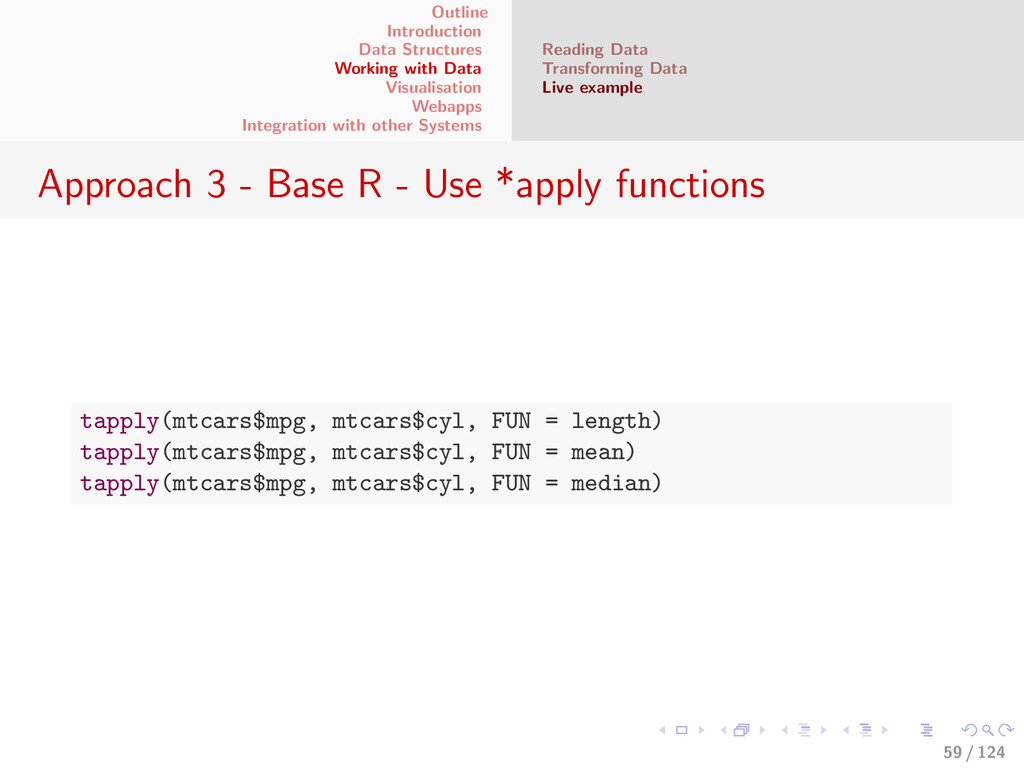
with other Systems Reading Data Transforming Data Live example Approach 3 - Base R - Use *apply functions tapply(mtcars$mpg, mtcars$cyl, FUN = length) tapply(mtcars$mpg, mtcars$cyl, FUN = mean) tapply(mtcars$mpg, mtcars$cyl, FUN = median) 59 / 124

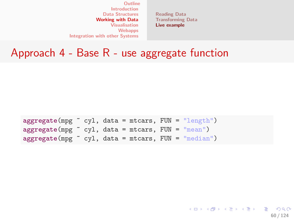
with other Systems Reading Data Transforming Data Live example Approach 4 - Base R - use aggregate function aggregate(mpg ~ cyl, data = mtcars, FUN = "length") aggregate(mpg ~ cyl, data = mtcars, FUN = "mean") aggregate(mpg ~ cyl, data = mtcars, FUN = "median") 60 / 124

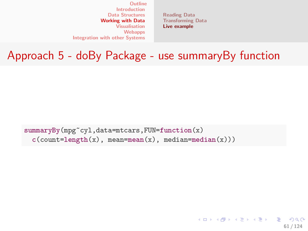
with other Systems Reading Data Transforming Data Live example Approach 5 - doBy Package - use summaryBy function summaryBy(mpg~cyl,data=mtcars,FUN=function(x) c(count=length(x), mean=mean(x), median=median(x))) 61 / 124

with other Systems Reading Data Transforming Data Live example Approach - plyr library - use **ply functions ddply(mtcars,'cyl',function(x) c(count=nrow(x), mean=mean(x$mpg), median=median(x$mpg)), .progress='text') 62 / 124

with other Systems Reading Data Transforming Data Live example More about the plyr module plyr is a very useful module for applying functions to diﬀerent datastructures. The functions in plyr are of the form XYply where ’X’ is the Input datatype and ’Y’ is the Output datatype So as in the above example, the input datatype was a dataframe and the output datatype is a dataframe. The type and their letter designations are a - array d - data.frame l - list m - matrix - no output returned 63 / 124

with other Systems Introduction Basic plots Advanced Plots Grammar of Graphics Outline 1 Introduction 2 Data Structures 3 Working with Data 4 Visualisation 5 Webapps 6 Integration with other Systems 64 / 124

with other Systems Introduction Basic plots Advanced Plots Grammar of Graphics Why Visualisation ? Easier to percieve diﬀerences easily (Magnitude, Range, Diﬀerence) Easier to see outliers, anomalier and grouping Easy to do exploratory analysis in R Easier to build narratives (Picture worth a million numbers) Bling !!! 65 / 124

with other Systems Introduction Basic plots Advanced Plots Grammar of Graphics Visualisation Packages boxplot, pie, hist from base graphics specialized packages like vioplot Grammar of Graphics - ggplot2 lattice 66 / 124

with other Systems Introduction Basic plots Advanced Plots Grammar of Graphics Boxplots Good for individual variable or groups of variables Good for showing outliers and quartiles (”shape”) take up less space than a histogram 67 / 124

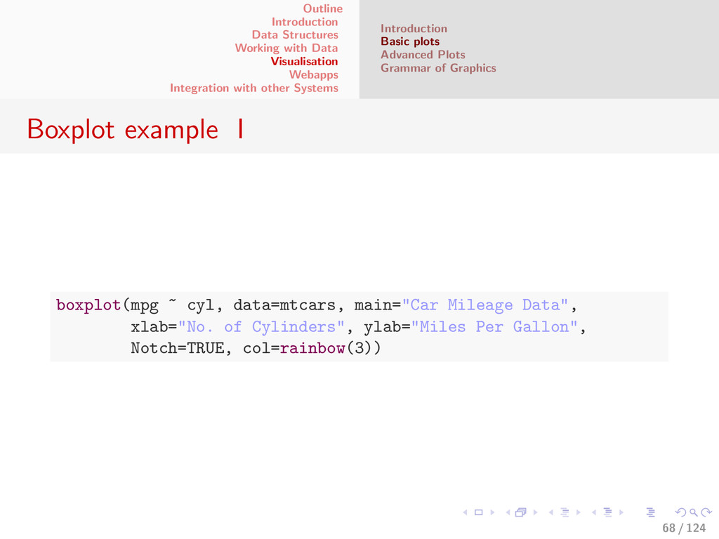
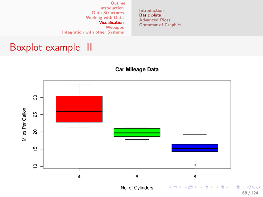
with other Systems Introduction Basic plots Advanced Plots Grammar of Graphics Boxplot example I boxplot(mpg ~ cyl, data=mtcars, main="Car Mileage Data", xlab="No. of Cylinders", ylab="Miles Per Gallon", Notch=TRUE, col=rainbow(3)) 68 / 124

with other Systems Introduction Basic plots Advanced Plots Grammar of Graphics Boxplot example II 4 6 8 10 15 20 25 30 Car Mileage Data No. of Cylinders Miles Per Gallon 69 / 124

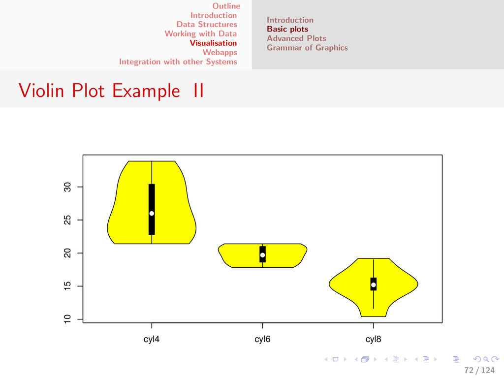
with other Systems Introduction Basic plots Advanced Plots Grammar of Graphics Violin plots Similar to boxplots but show probablity density Good for showing distribution Look like violins hence the name 70 / 124

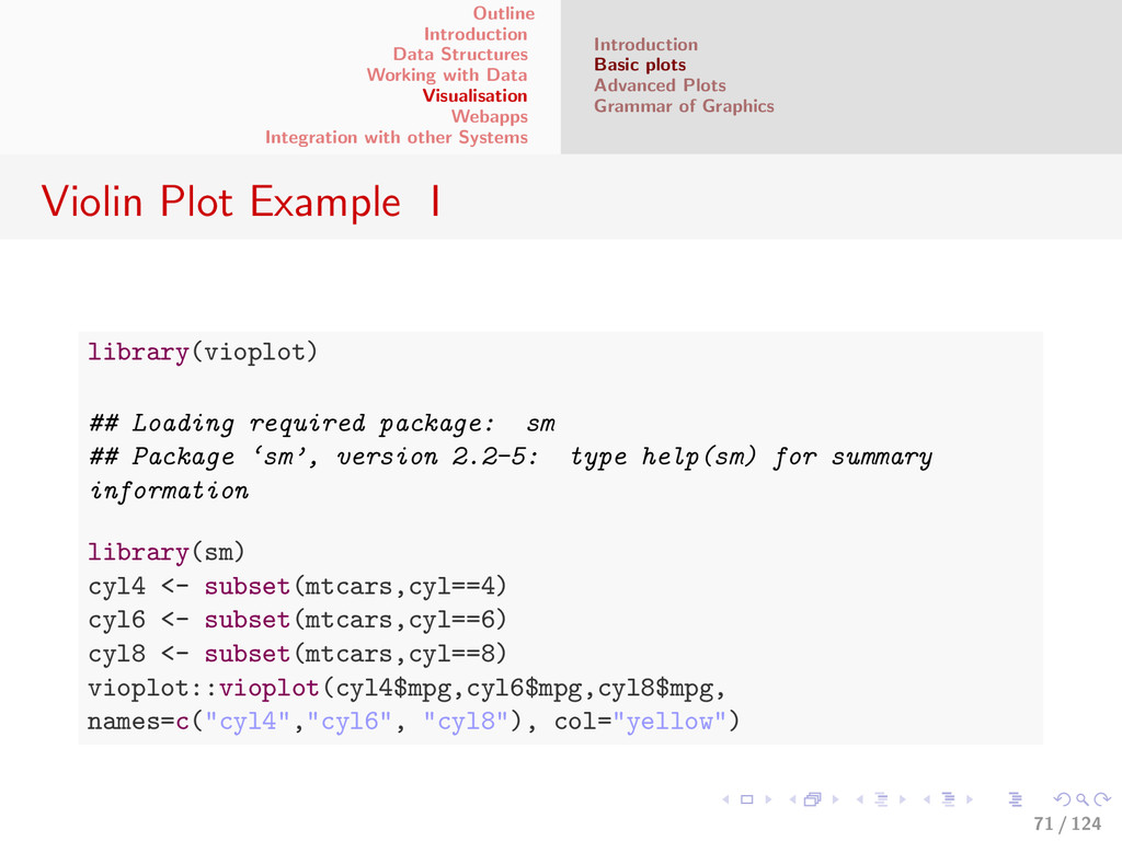
with other Systems Introduction Basic plots Advanced Plots Grammar of Graphics Violin Plot Example I library(vioplot) ## Loading required package: sm ## Package ‘sm’, version 2.2-5: type help(sm) for summary information library(sm) cyl4 <- subset(mtcars,cyl==4) cyl6 <- subset(mtcars,cyl==6) cyl8 <- subset(mtcars,cyl==8) vioplot::vioplot(cyl4$mpg,cyl6$mpg,cyl8$mpg, names=c("cyl4","cyl6", "cyl8"), col="yellow") 71 / 124

with other Systems Introduction Basic plots Advanced Plots Grammar of Graphics Violin Plot Example II 10 15 20 25 30 cyl4 cyl6 cyl8 72 / 124

with other Systems Introduction Basic plots Advanced Plots Grammar of Graphics Barplot Good to compare relative magnitudes Good to compare time series data Easier on the eyes 73 / 124

with other Systems Introduction Basic plots Advanced Plots Grammar of Graphics Barplot Example I barplot(table(mtcars$cyl),main="Car distribution", ylab="number of cylinders",xlab="Number of cars", horiz=TRUE,col=topo.colors(3)) 74 / 124

with other Systems Introduction Basic plots Advanced Plots Grammar of Graphics Barplot Example II 4 6 8 Car distribution Number of cars number of cylinders 0 2 4 6 8 10 12 14 75 / 124

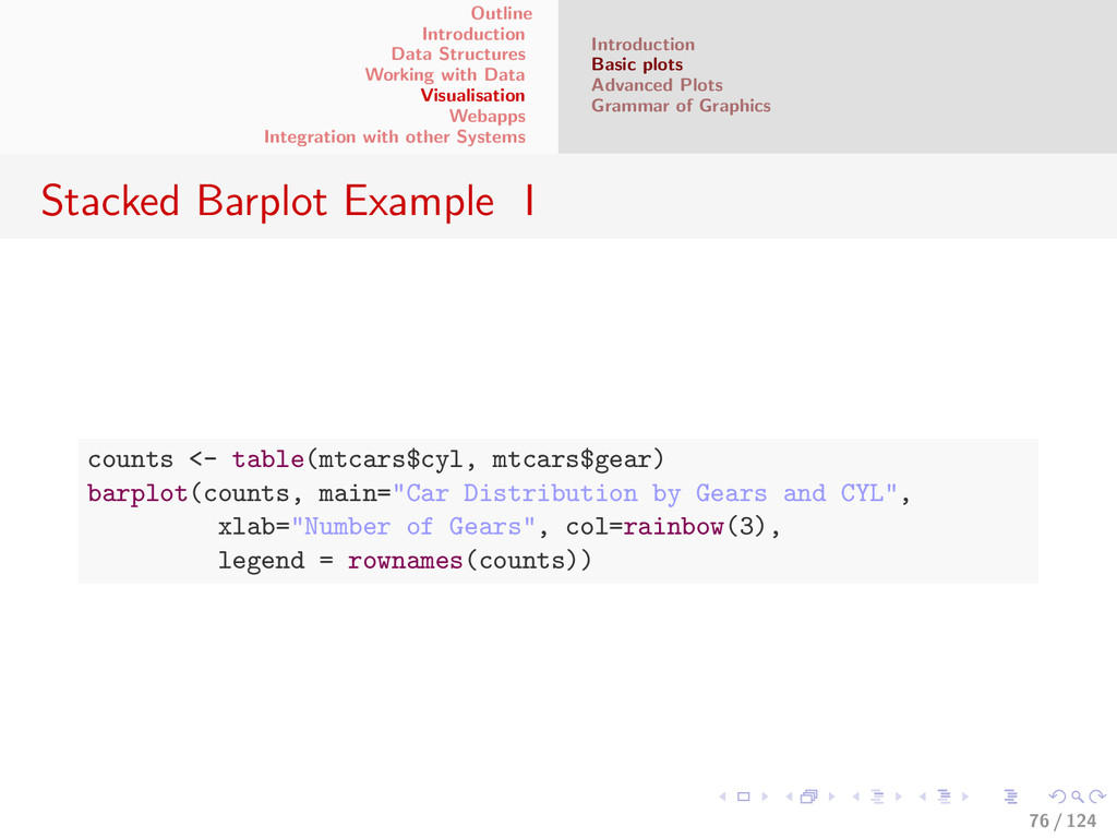
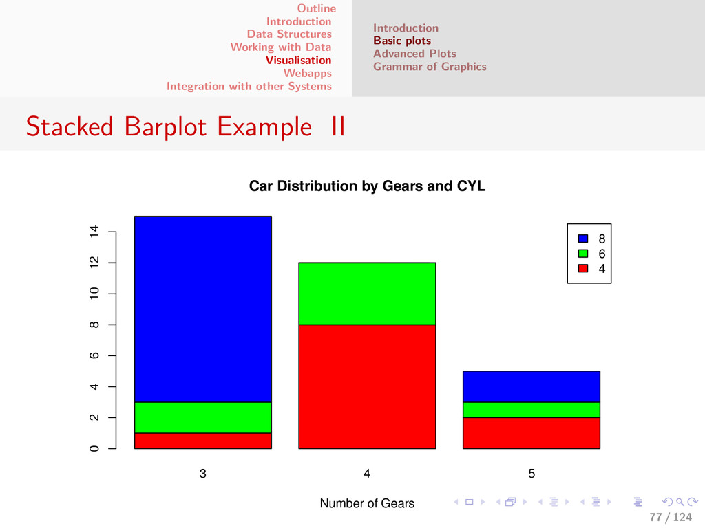
with other Systems Introduction Basic plots Advanced Plots Grammar of Graphics Stacked Barplot Example I counts <- table(mtcars$cyl, mtcars$gear) barplot(counts, main="Car Distribution by Gears and CYL", xlab="Number of Gears", col=rainbow(3), legend = rownames(counts)) 76 / 124

with other Systems Introduction Basic plots Advanced Plots Grammar of Graphics Stacked Barplot Example II 3 4 5 8 6 4 Car Distribution by Gears and CYL Number of Gears 0 2 4 6 8 10 12 14 77 / 124

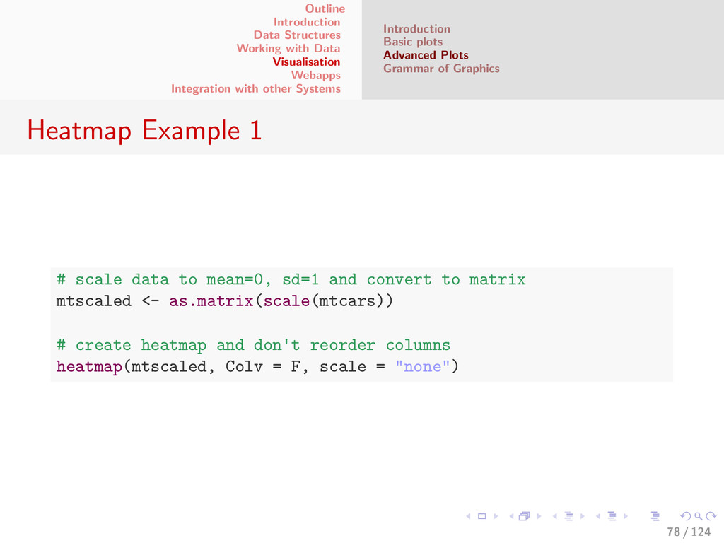
with other Systems Introduction Basic plots Advanced Plots Grammar of Graphics Heatmap Example 1 # scale data to mean=0, sd=1 and convert to matrix mtscaled <- as.matrix(scale(mtcars)) # create heatmap and don't reorder columns heatmap(mtscaled, Colv = F, scale = "none") 78 / 124

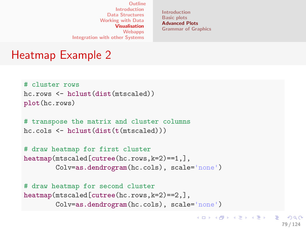
with other Systems Introduction Basic plots Advanced Plots Grammar of Graphics Heatmap Example 2 # cluster rows hc.rows <- hclust(dist(mtscaled)) plot(hc.rows) # transpose the matrix and cluster columns hc.cols <- hclust(dist(t(mtscaled))) # draw heatmap for first cluster heatmap(mtscaled[cutree(hc.rows,k=2)==1,], Colv=as.dendrogram(hc.cols), scale='none') # draw heatmap for second cluster heatmap(mtscaled[cutree(hc.rows,k=2)==2,], Colv=as.dendrogram(hc.cols), scale='none') 79 / 124

with other Systems Introduction Basic plots Advanced Plots Grammar of Graphics Introduction to ggplot2 Thinking about dataviz moves away from mechanics to representation Allows you to layer graphics and added remove components Based on Leland Wilkinson’s ”The Grammar of Graphics” book Allows to compose graphs based on components Allows to build beautiful graphs quickly 80 / 124

with other Systems Introduction Basic plots Advanced Plots Grammar of Graphics Components of Graphics - 1 Data - The cleaned up data with all the diﬀerent variables, factors. This includes the mappings to the aesthetic attributes of a plot. Geom - Geometric objects or geoms represent what you actually see on the screen. This includes lines, splines, points, polygons etc. Stat - Statistical transformations. These are optional. Examples include binning in a histogram or summarising a 2D relationship with a linear model. 81 / 124

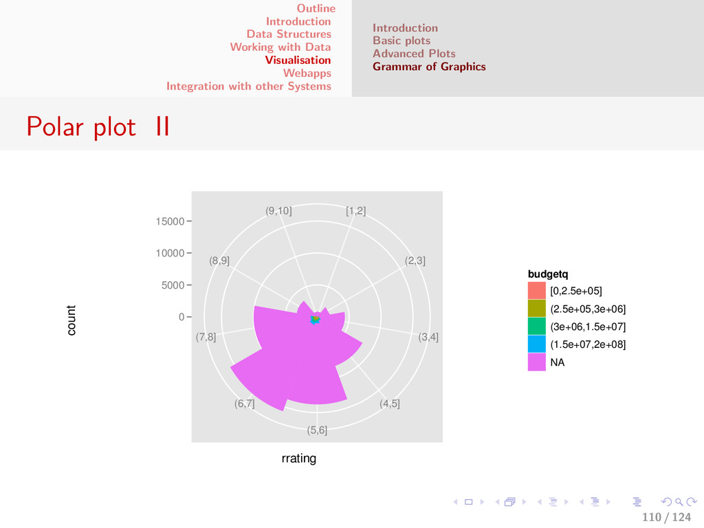
with other Systems Introduction Basic plots Advanced Plots Grammar of Graphics Components of Graphics - 2 Scale - Scales map values in the data into the aesthetic space such as color, size or shape. Scales draw axes and legends to represent what is seen on the screen to the actual underlying data. Coord - A coordinate sytems that provides a mapping from the data onto the screen. Examples include Cartesian coordinates, map coordinates and polar coordinates. Facet - A facet gives us a method to break un the data into subsets as well as display these on the screen. Great for increasing infomation density while graphing multidimensional data. 82 / 124

with other Systems Introduction Basic plots Advanced Plots Grammar of Graphics Scatterplot I library(ggplot2) qplot(displ, hwy, data = mpg) 83 / 124

with other Systems Introduction Basic plots Advanced Plots Grammar of Graphics Scatterplot II displ hwy 15 20 25 30 35 40 2 3 4 5 6 7 84 / 124

with other Systems Introduction Basic plots Advanced Plots Grammar of Graphics Scatterplot I qplot(displ, hwy, data = mpg, geom = "jitter") 85 / 124

with other Systems Introduction Basic plots Advanced Plots Grammar of Graphics Scatterplot II displ hwy 15 20 25 30 35 40 2 3 4 5 6 7 86 / 124

with other Systems Introduction Basic plots Advanced Plots Grammar of Graphics Scatterplot I qplot(displ, hwy, data = mpg, color = class) 87 / 124

with other Systems Introduction Basic plots Advanced Plots Grammar of Graphics Scatterplot II displ hwy 15 20 25 30 35 40 2 3 4 5 6 7 class 2seater compact midsize minivan pickup subcompact suv 88 / 124

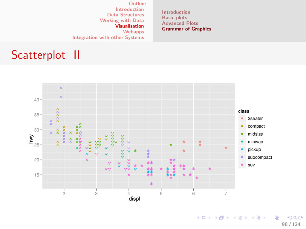
with other Systems Introduction Basic plots Advanced Plots Grammar of Graphics Scatterplot I qplot(displ, hwy, data = mpg, color = class, shape = cyl) 89 / 124

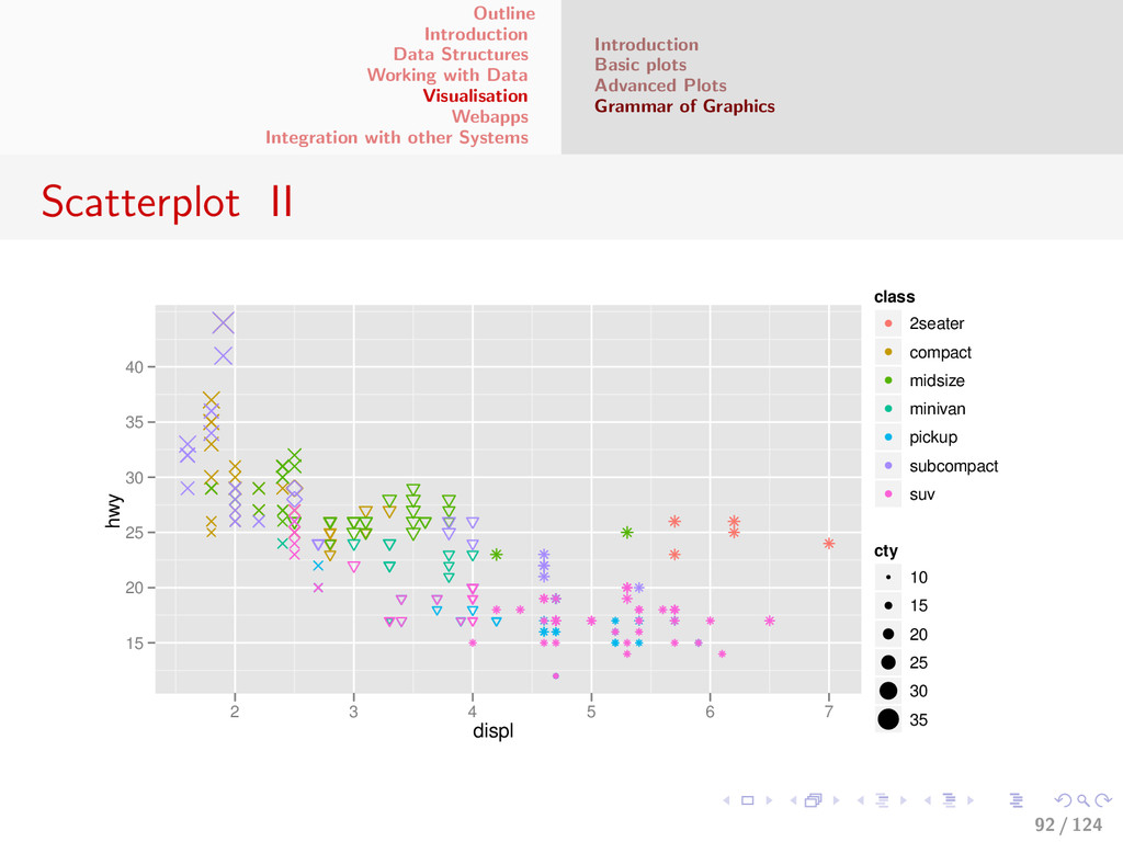
with other Systems Introduction Basic plots Advanced Plots Grammar of Graphics Scatterplot II displ hwy 15 20 25 30 35 40 2 3 4 5 6 7 class 2seater compact midsize minivan pickup subcompact suv 90 / 124

with other Systems Introduction Basic plots Advanced Plots Grammar of Graphics Scatterplot I qplot(displ, hwy, data = mpg, color = class, shape = cyl, size = cty) 91 / 124

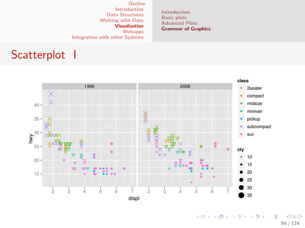
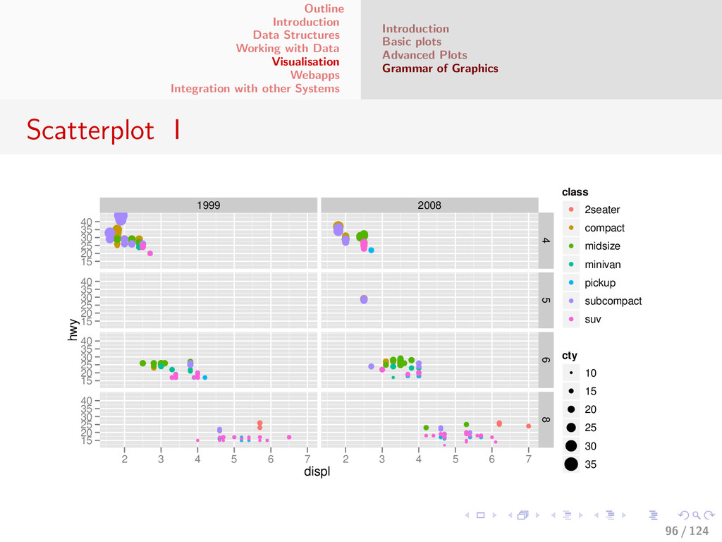
with other Systems Introduction Basic plots Advanced Plots Grammar of Graphics Scatterplot II displ hwy 15 20 25 30 35 40 2 3 4 5 6 7 class 2seater compact midsize minivan pickup subcompact suv cty 10 15 20 25 30 35 92 / 124

with other Systems Introduction Basic plots Advanced Plots Grammar of Graphics Scatterplot I qplot(displ,hwy,data=mpg,color=class,shape=cyl,size=cty) + facet_wrap (~year) 93 / 124

with other Systems Introduction Basic plots Advanced Plots Grammar of Graphics Scatterplot I displ hwy 15 20 25 30 35 40 1999 2 3 4 5 6 7 2008 2 3 4 5 6 7 class 2seater compact midsize minivan pickup subcompact suv cty 10 15 20 25 30 35 94 / 124

with other Systems Introduction Basic plots Advanced Plots Grammar of Graphics Scatterplot I qplot(displ, hwy, data = mpg, color = class, shape = cyl, size = cty) +facet_wrap(~year) 95 / 124

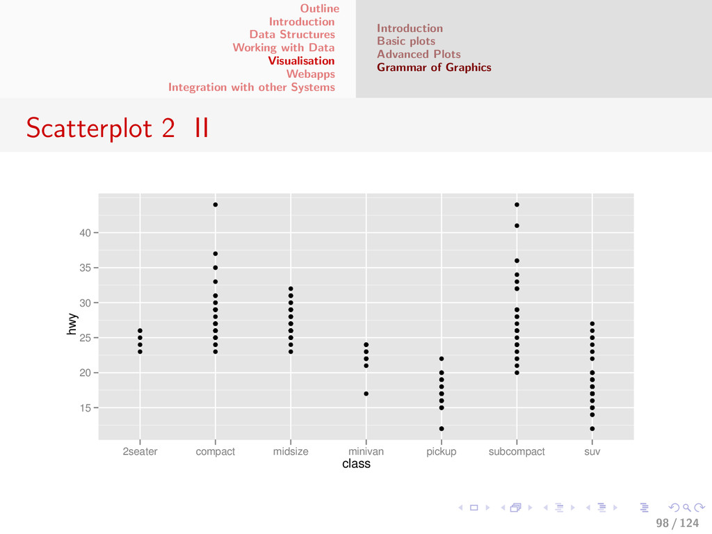
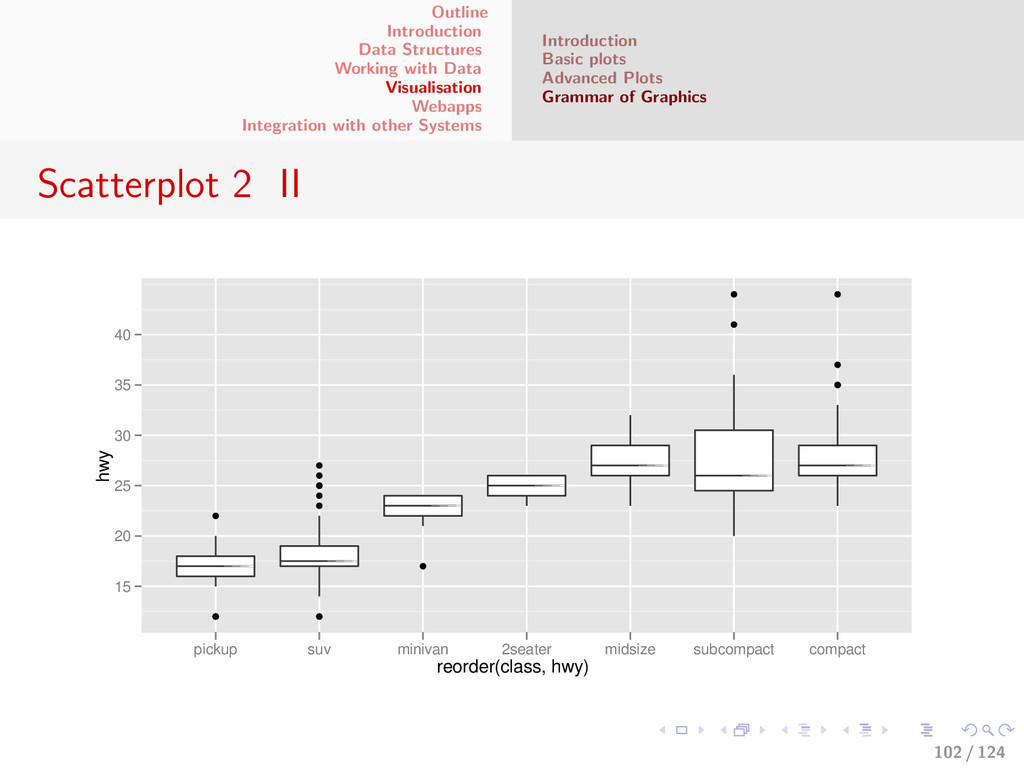
with other Systems Introduction Basic plots Advanced Plots Grammar of Graphics Scatterplot I displ hwy 15 20 25 30 35 40 15 20 25 30 35 40 15 20 25 30 35 40 15 20 25 30 35 40 1999 2 3 4 5 6 7 2008 2 3 4 5 6 7 4 5 6 8 class 2seater compact midsize minivan pickup subcompact suv cty 10 15 20 25 30 35 96 / 124

with other Systems Introduction Basic plots Advanced Plots Grammar of Graphics Scatterplot 2 I qplot(class, hwy, data = mpg) 97 / 124

with other Systems Introduction Basic plots Advanced Plots Grammar of Graphics Scatterplot 2 II class hwy 15 20 25 30 35 40 2seater compact midsize minivan pickup subcompact suv 98 / 124

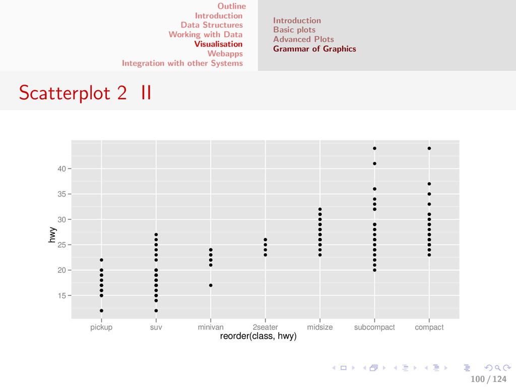
with other Systems Introduction Basic plots Advanced Plots Grammar of Graphics Scatterplot 2 I qplot(reorder(class, hwy), hwy, data = mpg) 99 / 124

with other Systems Introduction Basic plots Advanced Plots Grammar of Graphics Scatterplot 2 II reorder(class, hwy) hwy 15 20 25 30 35 40 pickup suv minivan 2seater midsize subcompact compact 100 / 124

with other Systems Introduction Basic plots Advanced Plots Grammar of Graphics Scatterplot 2 I qplot(reorder(class, hwy), hwy, data = mpg, geom="boxplot") 101 / 124

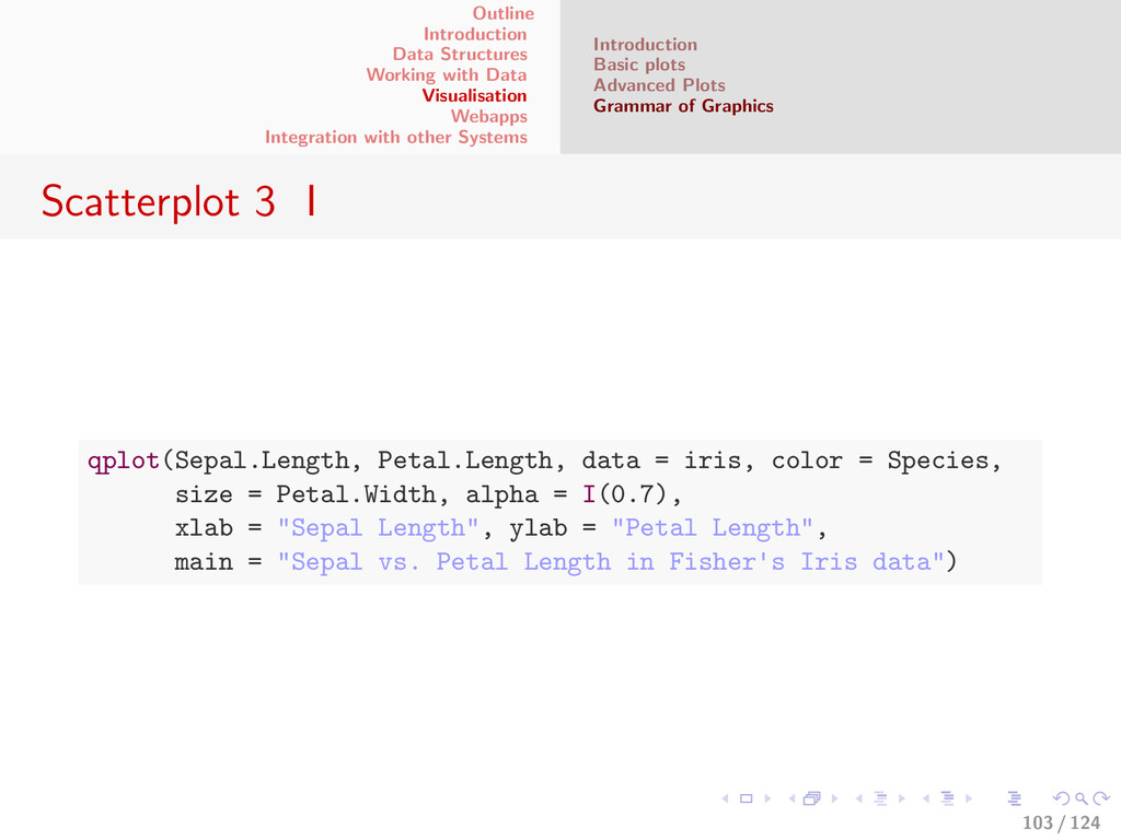
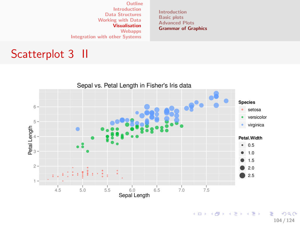
with other Systems Introduction Basic plots Advanced Plots Grammar of Graphics Scatterplot 2 II reorder(class, hwy) hwy 15 20 25 30 35 40 pickup suv minivan 2seater midsize subcompact compact 102 / 124

with other Systems Introduction Basic plots Advanced Plots Grammar of Graphics Scatterplot 3 I qplot(Sepal.Length, Petal.Length, data = iris, color = Species, size = Petal.Width, alpha = I(0.7), xlab = "Sepal Length", ylab = "Petal Length", main = "Sepal vs. Petal Length in Fisher's Iris data") 103 / 124

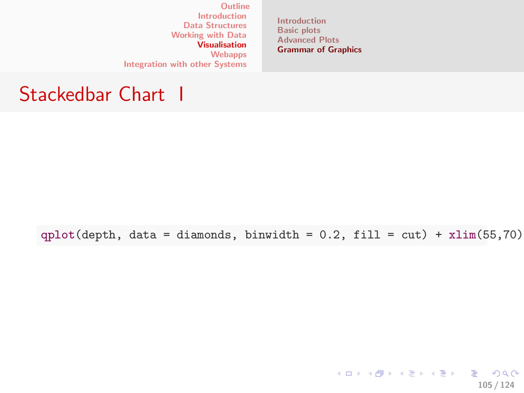
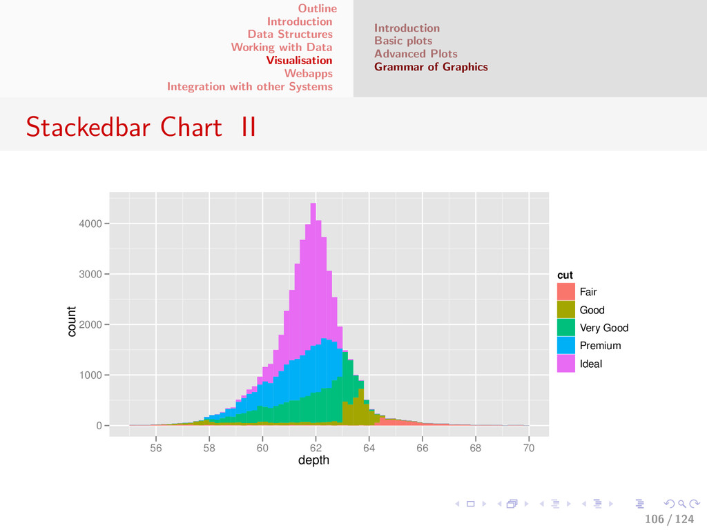
with other Systems Introduction Basic plots Advanced Plots Grammar of Graphics Scatterplot 3 II Sepal vs. Petal Length in Fisher's Iris data Sepal Length Petal Length 1 2 3 4 5 6 4.5 5.0 5.5 6.0 6.5 7.0 7.5 Species setosa versicolor virginica Petal.Width 0.5 1.0 1.5 2.0 2.5 104 / 124

with other Systems Introduction Basic plots Advanced Plots Grammar of Graphics Stackedbar Chart I qplot(depth, data = diamonds, binwidth = 0.2, fill = cut) + xlim(55,70) 105 / 124

with other Systems Introduction Basic plots Advanced Plots Grammar of Graphics Stackedbar Chart II depth count 0 1000 2000 3000 4000 56 58 60 62 64 66 68 70 cut Fair Good Very Good Premium Ideal 106 / 124

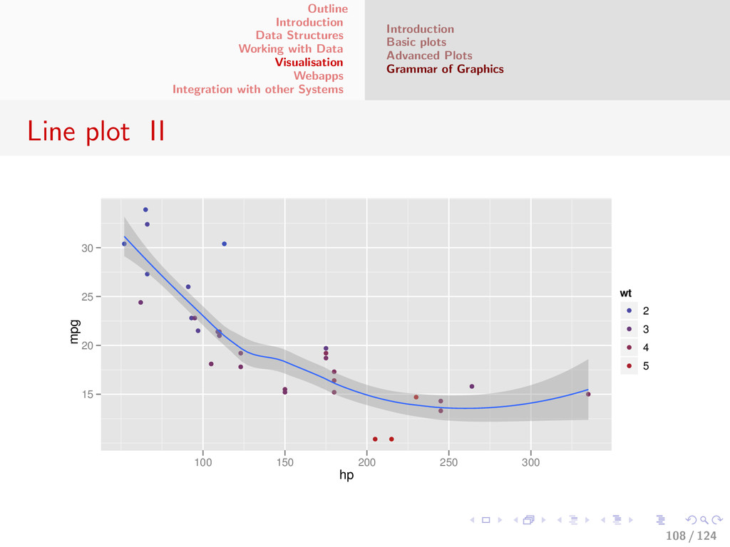
with other Systems Introduction Basic plots Advanced Plots Grammar of Graphics Line plot I # Scale + Layering + Aesthetic example plotl <- ggplot(mtcars, aes(x=hp,y=mpg)) plotl + geom_point(aes(color=wt)) + geom_smooth() 107 / 124

with other Systems Introduction Basic plots Advanced Plots Grammar of Graphics Line plot II hp mpg 15 20 25 30 100 150 200 250 300 wt 2 3 4 5 108 / 124

with other Systems Introduction Basic plots Advanced Plots Grammar of Graphics Polar plot I # from ggplot2 docs # Windrose + doughnut plot movies$rrating <- cut_interval(movies$rating, length = 1) movies$budgetq <- cut_number(movies$budget, 4) doh <- ggplot(movies, aes(x = rrating, fill = budgetq)) # Wind rose doh + geom_bar(width = 1) + coord_polar() 109 / 124

with other Systems Introduction Basic plots Advanced Plots Grammar of Graphics Polar plot II rrating count 0 5000 10000 15000 [1,2] (2,3] (3,4] (4,5] (5,6] (6,7] (7,8] (8,9] (9,10] budgetq [0,2.5e+05] (2.5e+05,3e+06] (3e+06,1.5e+07] (1.5e+07,2e+08] NA 110 / 124

with other Systems Introduction Basic plots Advanced Plots Grammar of Graphics Cons of Grammar of Graphics Grammar doesn’t specify ﬁner points of graphing such os font size or background color. GGplot2 Themes tries to mitigate this) Great for static graphs but not good for interactivity or animation. There are workarounds for this though. 111 / 124

with other Systems Introduction to Shiny Features Architecture Code example Outline 1 Introduction 2 Data Structures 3 Working with Data 4 Visualisation 5 Webapps 6 Integration with other Systems 112 / 124

with other Systems Introduction to Shiny Features Architecture Code example Shiny Shiny package from Rstudio Shiny is a new package from RStudio that makes it incredibly easy to build interactive web applications with R. 113 / 124

with other Systems Introduction to Shiny Features Architecture Code example Features Build useful web applications with only a few lines of codeno JavaScript required. Shiny user interfaces can be built entirely using R, or integrated with HTML, CSS, and JavaScript for more ﬂexibility. Works in any R environment (Console R, Rgui for Windows or Mac, ESS, StatET, RStudio, etc.) 114 / 124

with other Systems Introduction to Shiny Features Architecture Code example Features Pre-built output widgets for displaying plots, tables, and printed output of R objects. Fast bidirectional communication between the web browser and R using the websockets package. Uses a reactive programming model that eliminates messy event handling code, so you can focus on the code that really matters. 115 / 124

with other Systems Introduction to Shiny Features Architecture Code example Architecture and Code Layout Shiny applications have two components - A user-interface definition script and server script It follows event-based programming model - Anytime any UI component is changed such as selection or movemnet of slider, an event is fired to the backend to handle. Server and client communicate seamlessly using websockets. An event triggers a server response and the UI is refreshed accordingly to reflect the change. 116 / 124

with other Systems Introduction to Shiny Features Architecture Code example A live plot of mpg dataset 117 / 124

with other Systems Outline 1 Introduction 2 Data Structures 3 Working with Data 4 Visualisation 5 Webapps 6 Integration with other Systems 118 / 124

with other Systems Packages hadoop - RHadoop c++ - RCpp javascript - Shiny 119 / 124

with other Systems Literate programming using Knitr Literate programming Literate programming is an approach to programming introduced by Donald Knuth in which a program is given as an explanation of the program logic in a natural language, such as English, interspersed with snippets of macros and traditional source code, from which a compilable source code can be generated 120 / 124

with other Systems Knitr Transparent engine for dynamic report generation with R Implements literate programming paradigm Only one document to edit. Less pain to keep everything in sync Can output into diﬀerent ﬁnal outputs such as HTML, PDF etc 121 / 124

with other Systems Knitr features Faithful output Built-in cache Easy Formatting Flexibility in output devices 122 / 124

with other Systems Knitr Demo 123 / 124

with other Systems Thank you Twitter @vinayakh Email vinayakh at gmail 124 / 124

Introduction to Data Analysis and Visualization...

Introduction to Data Analysis and Visualization using R

More Decks by Vinayak

Other Decks in Technology

Featured

Transcript