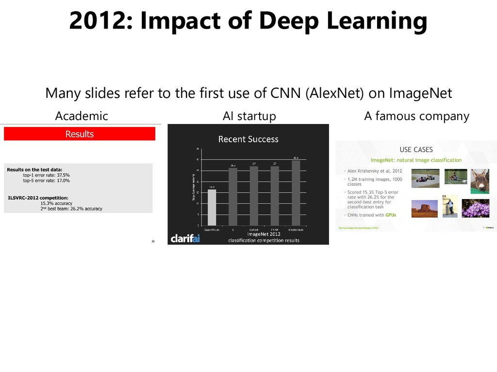
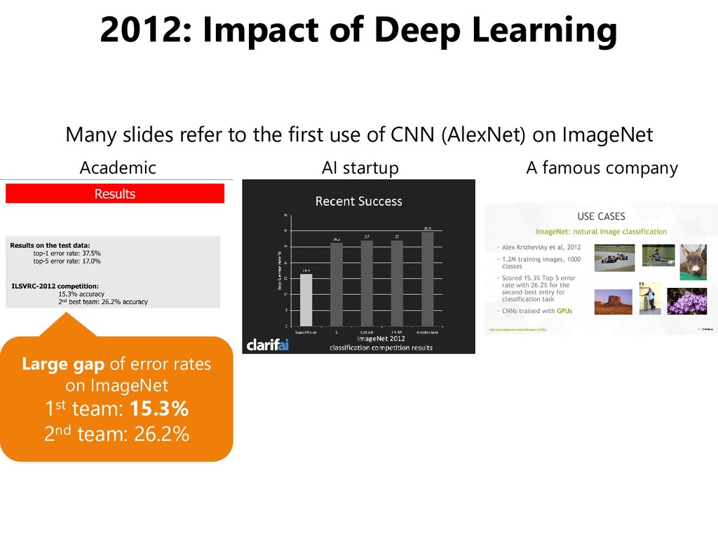
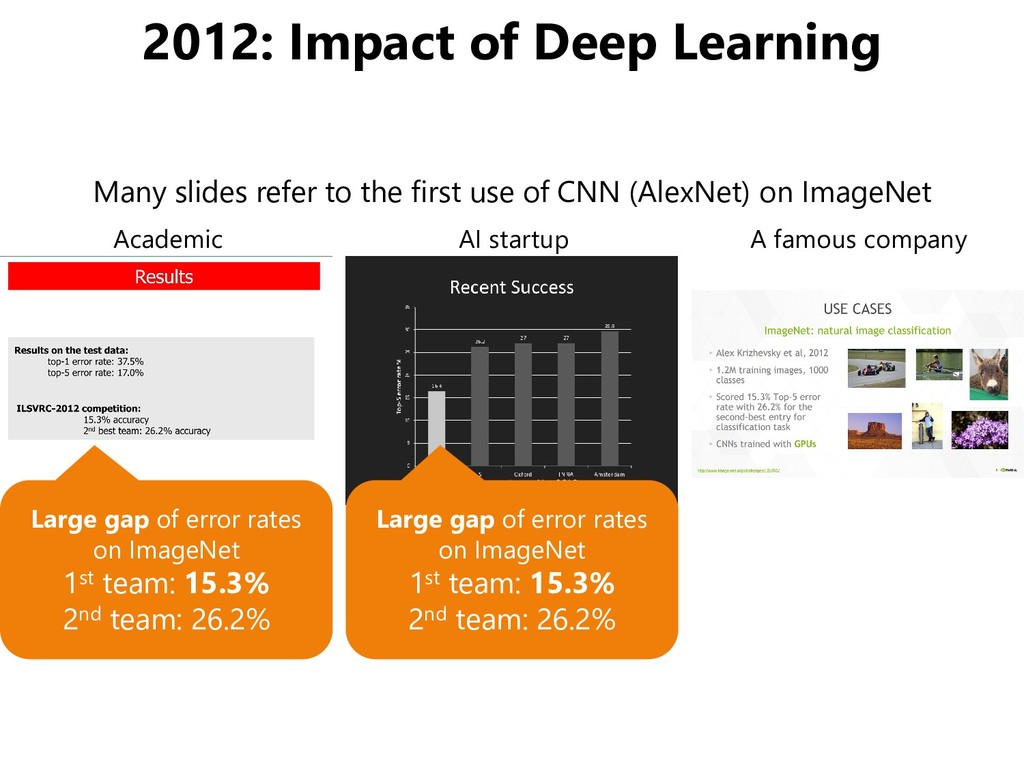
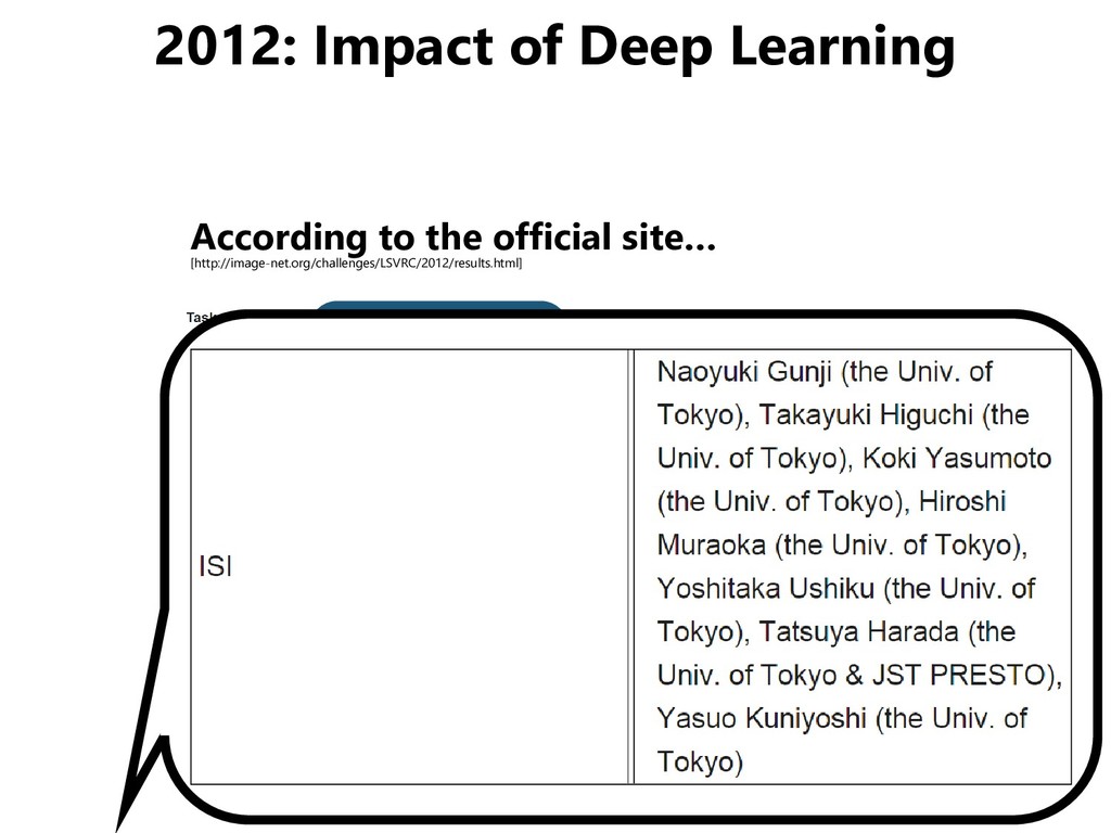
company Large gap of error rates on ImageNet 1st team: 15.3% 2nd team: 26.2% Large gap of error rates on ImageNet 1st team: 15.3% 2nd team: 26.2% Many slides refer to the first use of CNN (AlexNet) on ImageNet
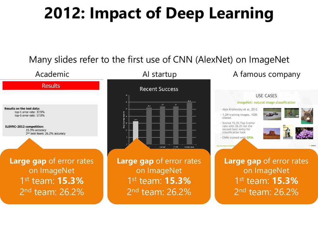
company Large gap of error rates on ImageNet 1st team: 15.3% 2nd team: 26.2% Large gap of error rates on ImageNet 1st team: 15.3% 2nd team: 26.2% Large gap of error rates on ImageNet 1st team: 15.3% 2nd team: 26.2% Many slides refer to the first use of CNN (AlexNet) on ImageNet
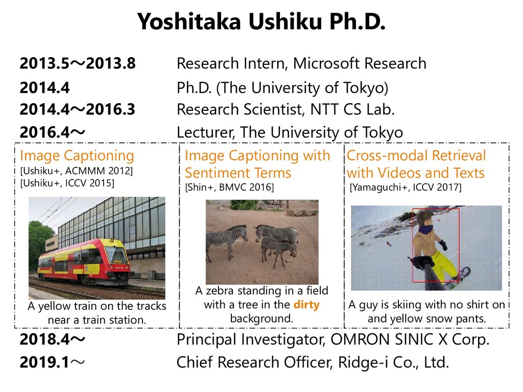
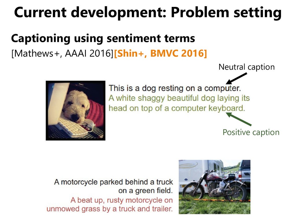
(The University of Tokyo) 2014.4~2016.3 Research Scientist, NTT CS Lab. 2016.4~ Lecturer, The University of Tokyo 2018.4~ Principal Investigator, OMRON SINIC X Corp. 2019.1~ Chief Research Officer, Ridge-i Co., Ltd. [Ushiku+, ACMMM 2012] [Ushiku+, ICCV 2015] Image Captioning Image Captioning with Sentiment Terms Cross-modal Retrieval with Videos and Texts [Yamaguchi+, ICCV 2017] A guy is skiing with no shirt on and yellow snow pants. A zebra standing in a field with a tree in the dirty background. [Shin+, BMVC 2016] A yellow train on the tracks near a train station.
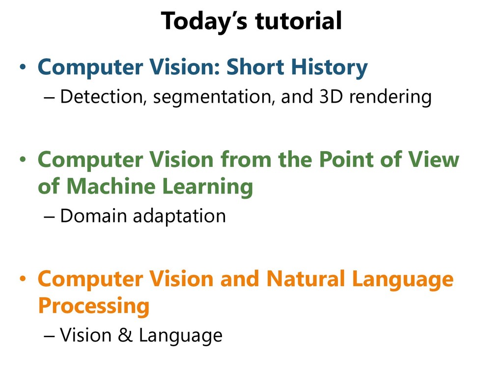
and 3D rendering • Computer Vision from the Point of View of Machine Learning – Domain adaptation • Computer Vision and Natural Language Processing – Vision & Language
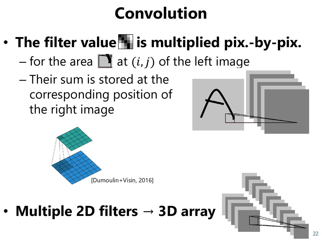
the area at (, ) of the left image – Their sum is stored at the corresponding position of the right image • Multiple 2D filters → 3D array 22 [Dumoulin+Visin, 2016]
by Oxford's Visual Geometry Group – “Depth“ is highlighted • Inception [Szegedy, CVPR 2015] – CNN by Google – Inception Block (right bottom) is applied repeatedly. – After reducing the number of channels by 1x1 convolution, 3x3 or 5x5 convolution is applied → high expressiveness with fewer parameters 24
region proposal from an image – CNN over each region • Faster RCNN [Ren+, NIPS 2015] – RCNN requires multiple calculation of CNN for a single image – Faster RCNN: Apply CNN only once to the whole image and estimate candidate area at the same time → High speed and precision 26
skip connection – The finer parts of each region can be segmented precisely • DeepLab v3[Chen+, ECCV 2018] – Feature extraction from multiple resolution – Skip connection
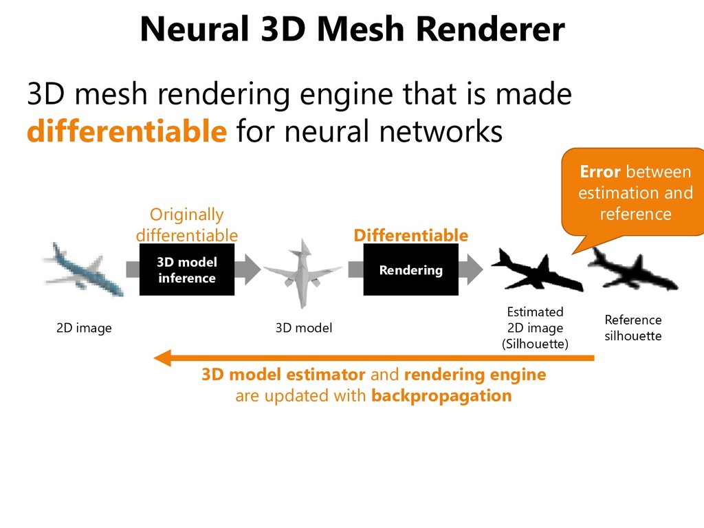
made differentiable for neural networks 3D model inference Rendering Error between estimation and reference 2D image 3D model Estimated 2D image (Silhouette) Reference silhouette 3D model estimator and rendering engine are updated with backpropagation Originally differentiable Differentiable
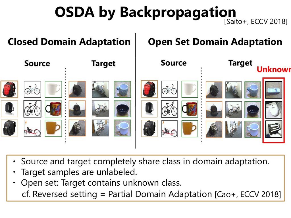
with ground truth, but we don’t want to recognize them as an application. • Target Domain: We want to recognize them, but there are no data associated with ground truth. • Semi-supervised Domain Adaptation: There are some target samples with ground truth. Video Game Real World
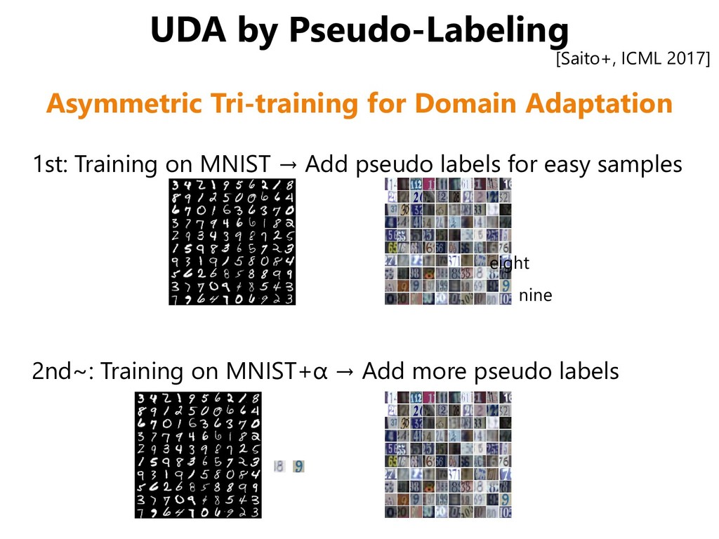
labels for easy samples 2nd~: Training on MNIST+α → Add more pseudo labels eight nine Asymmetric Tri-training for Domain Adaptation [Saito+, ICML 2017]
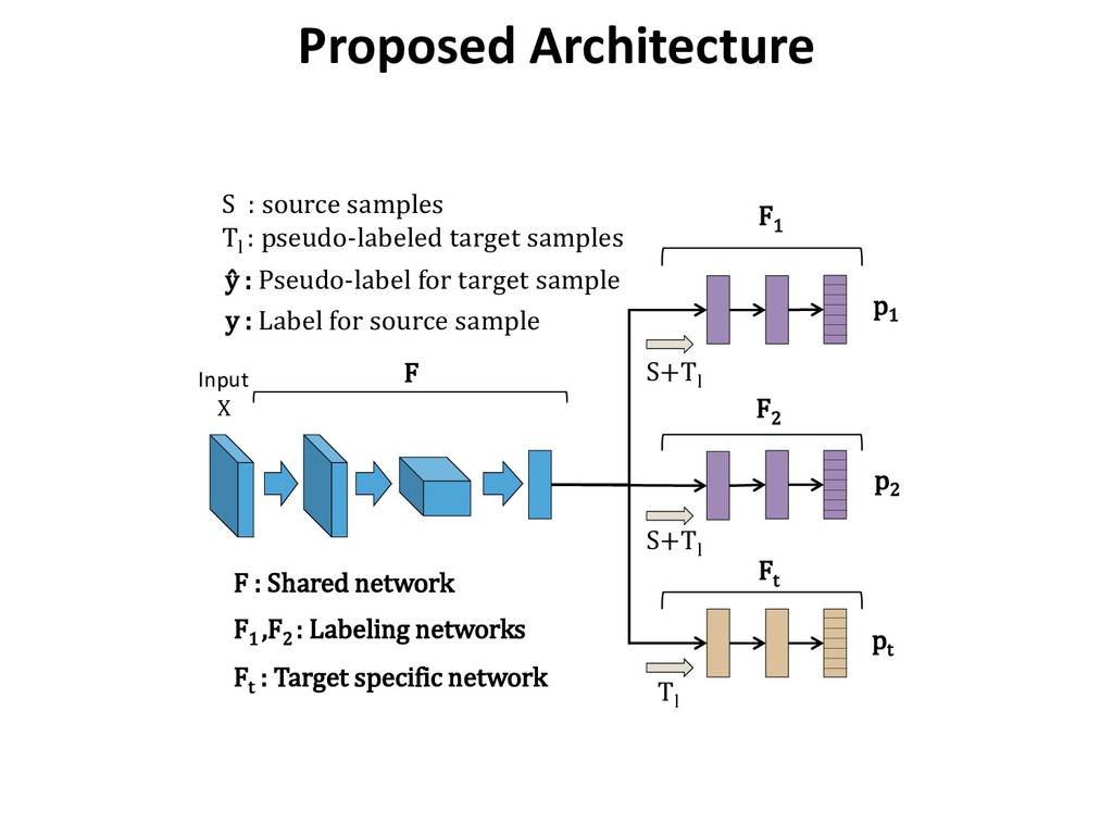
: pseudo-labeled target samples Input X F1 F2 Ft ŷ : Pseudo-label for target sample y : Label for source sample F S+Tl F1 ,F2 : Labeling networks Ft : Target specific network F : Shared network Proposed Architecture
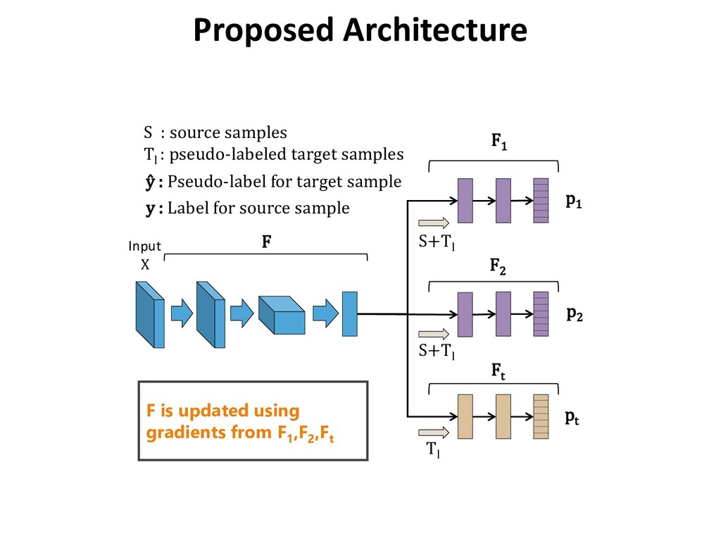
: pseudo-labeled target samples Input X F1 F2 Ft ŷ : Pseudo-label for target sample y : Label for source sample F S+Tl F is updated using gradients from F1 ,F2 ,Ft Proposed Architecture
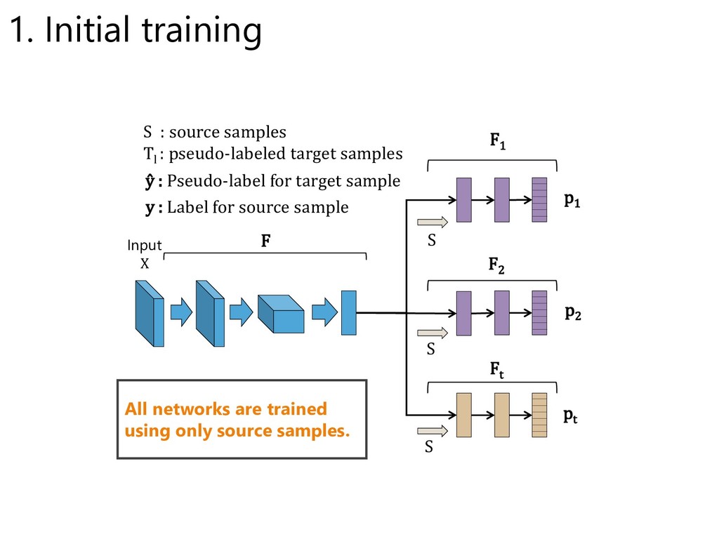
: pseudo-labeled target samples Input X F1 F2 Ft ŷ : Pseudo-label for target sample y : Label for source sample F S All networks are trained using only source samples. 1. Initial training
F1 and F2 agree on their predictions, and either of their probability is larger than threshold value, corresponding labels are given to the target sample. T: Target samples 2. Labeling target samples
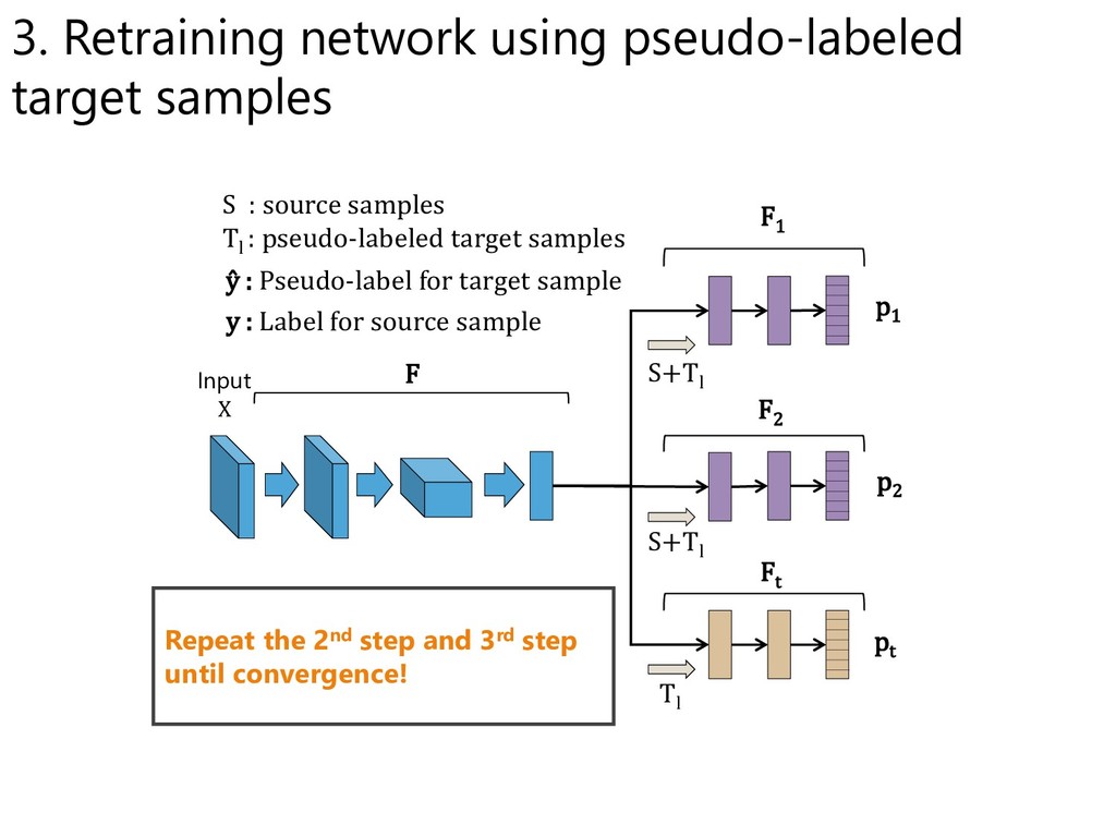
pseudo-labeled ones F : learn from all gradients p1 p2 pt S+Tl Tl S : source samples Tl : pseudo-labeled target samples Input X F1 F2 Ft ŷ : Pseudo-label for target sample y : Label for source sample F S+Tl 3. Retraining network using pseudo-labeled target samples
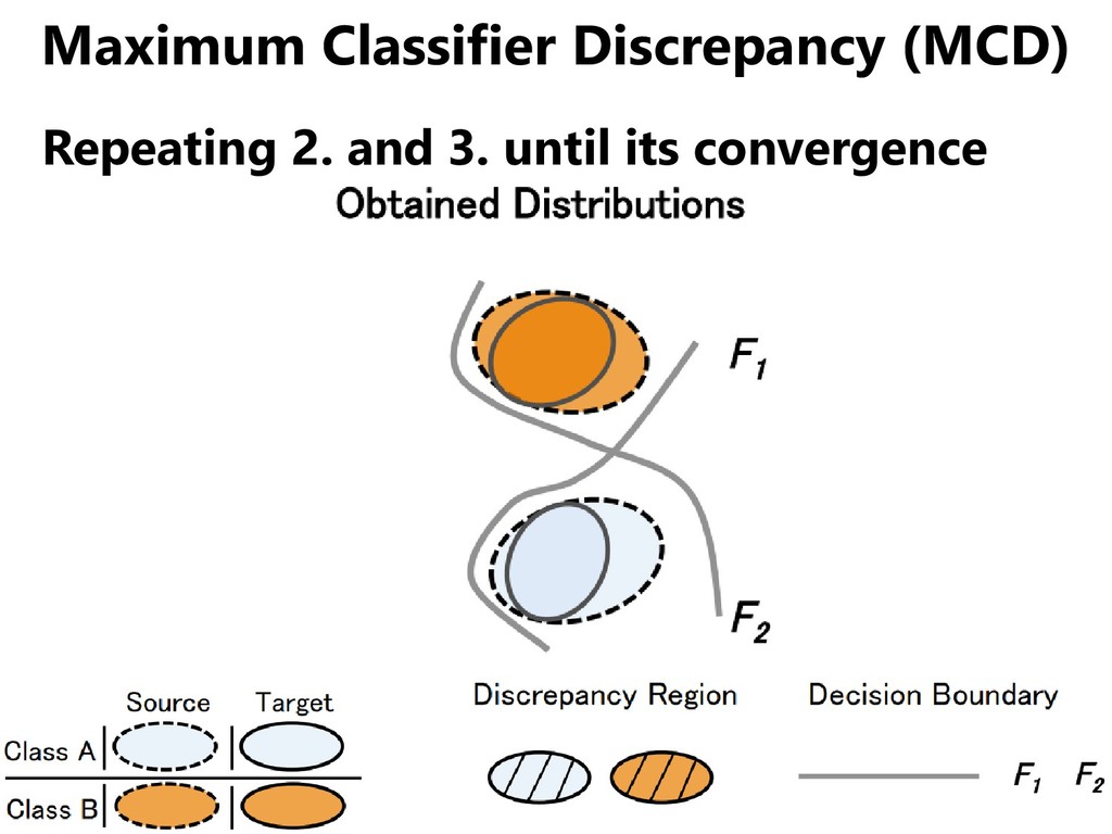
: pseudo-labeled target samples Input X F1 F2 Ft ŷ : Pseudo-label for target sample y : Label for source sample F S+Tl Repeat the 2nd step and 3rd step until convergence! 3. Retraining network using pseudo-labeled target samples
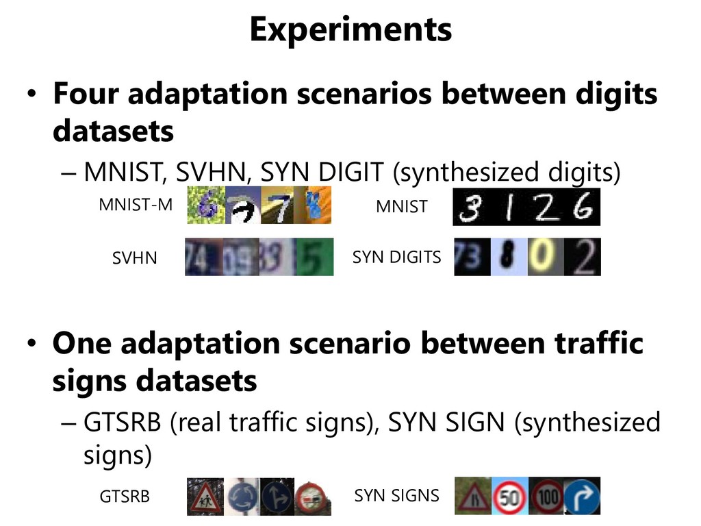
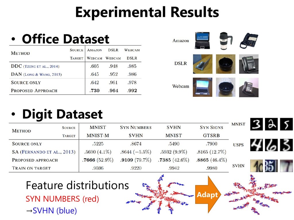
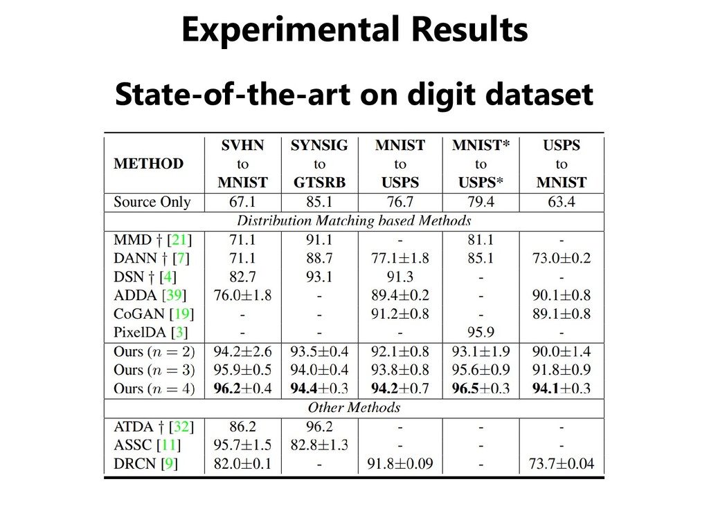
SVHN, SYN DIGIT (synthesized digits) • One adaptation scenario between traffic signs datasets – GTSRB (real traffic signs), SYN SIGN (synthesized signs) GTSRB SYN SIGNS SYN DIGITS SVHN MNIST MNIST-M
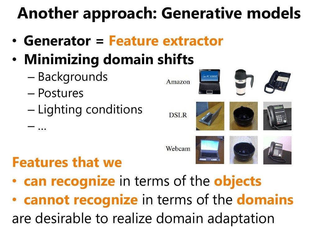
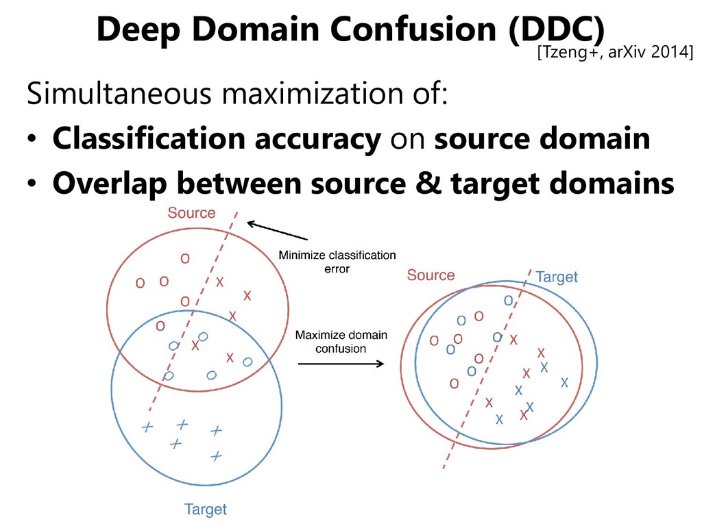
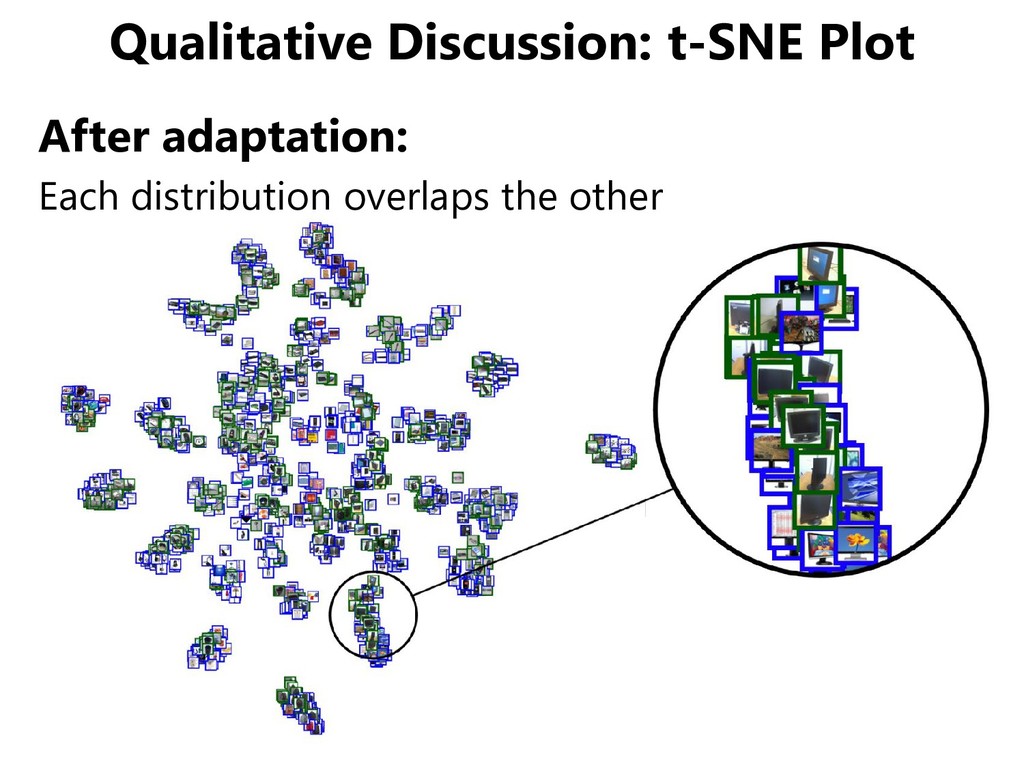
Minimizing domain shifts – Backgrounds – Postures – Lighting conditions – … Features that we • can recognize in terms of the objects • cannot recognize in terms of the domains are desirable to realize domain adaptation
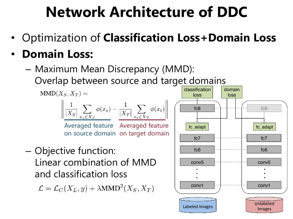
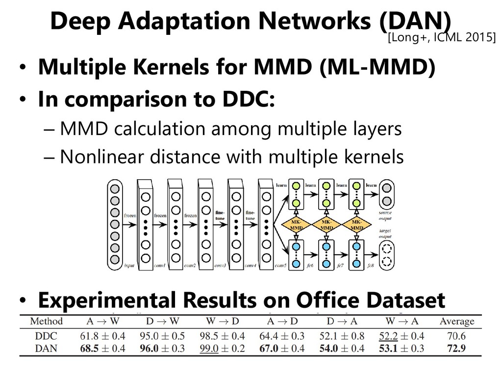
• Domain Loss: – Maximum Mean Discrepancy (MMD): Overlap between source and target domains – Objective function: Linear combination of MMD and classification loss Averaged feature on source domain Averaged feature on target domain
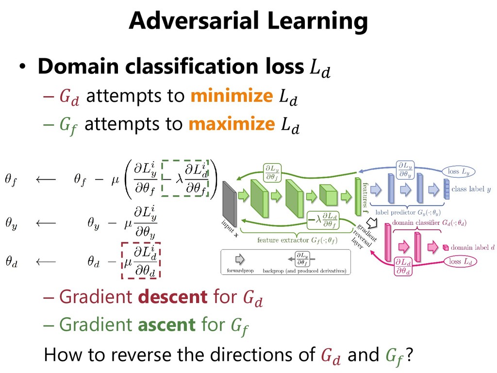
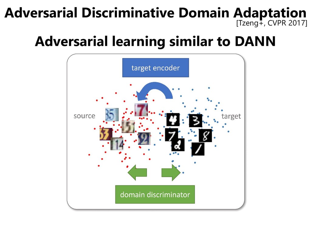
include “adversarial” – The name “Domain Adversarial Neural Networks” appears in the journal version [Ganin+, JMLR 2016] – Maybe confused with Deep Adaptation Networks (DAN) • Similar motivation to GANs: Adversarial learning to generate (extract) domain-invariant feature vectors – GAN: generated data vs. real data – DANN: feature vectors on a source domain vs. feature vectors on a target domain [Ganin+Lempitsky, ICML 2015]
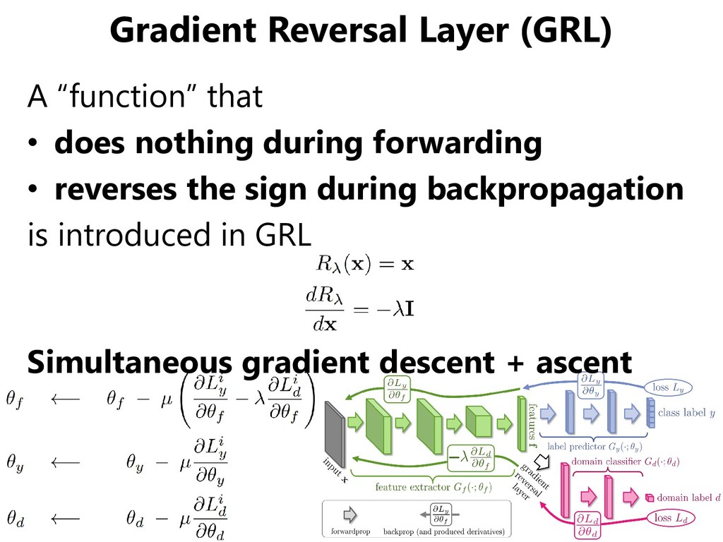
for both domains ✓The number of parameters can be reduced ×It might be impossible to extract features of different domains using the same extractor. • Gradient Reversal Layer ✓It is faithful to the objective function of GANs ×Gradients from the discriminator may be vanished early in the training
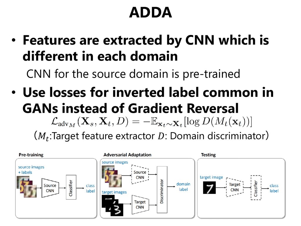
in each domain CNN for the source domain is pre-trained • Use losses for inverted label common in GANs instead of Gradient Reversal ( :Target feature extractor : Domain discriminator)
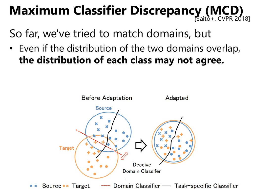
domains, but • Even if the distribution of the two domains overlap, the distribution of each class may not agree. • We should match classifiers instead of domains. [Saito+, CVPR 2018]
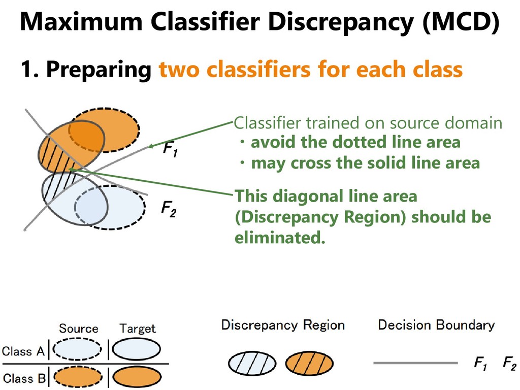
class Classifier trained on source domain ・avoid the dotted line area ・may cross the solid line area This diagonal line area (Discrepancy Region) should be eliminated.
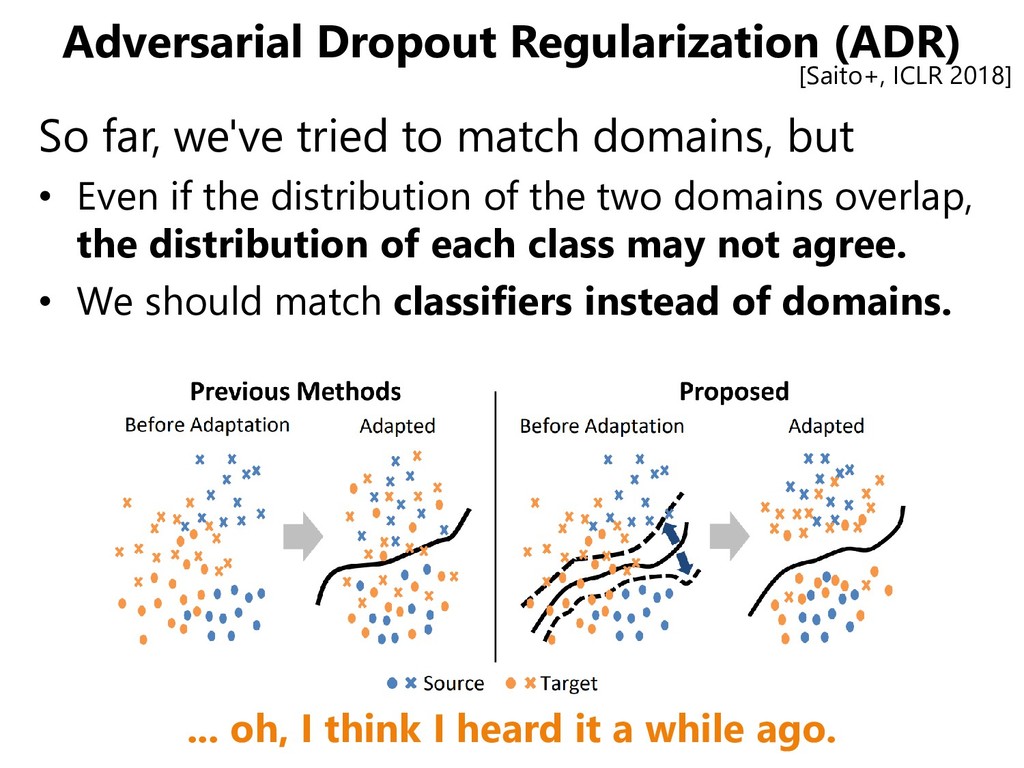
domains, but • Even if the distribution of the two domains overlap, the distribution of each class may not agree. • We should match classifiers instead of domains. [Saito+, ICLR 2018] ... oh, I think I heard it a while ago.
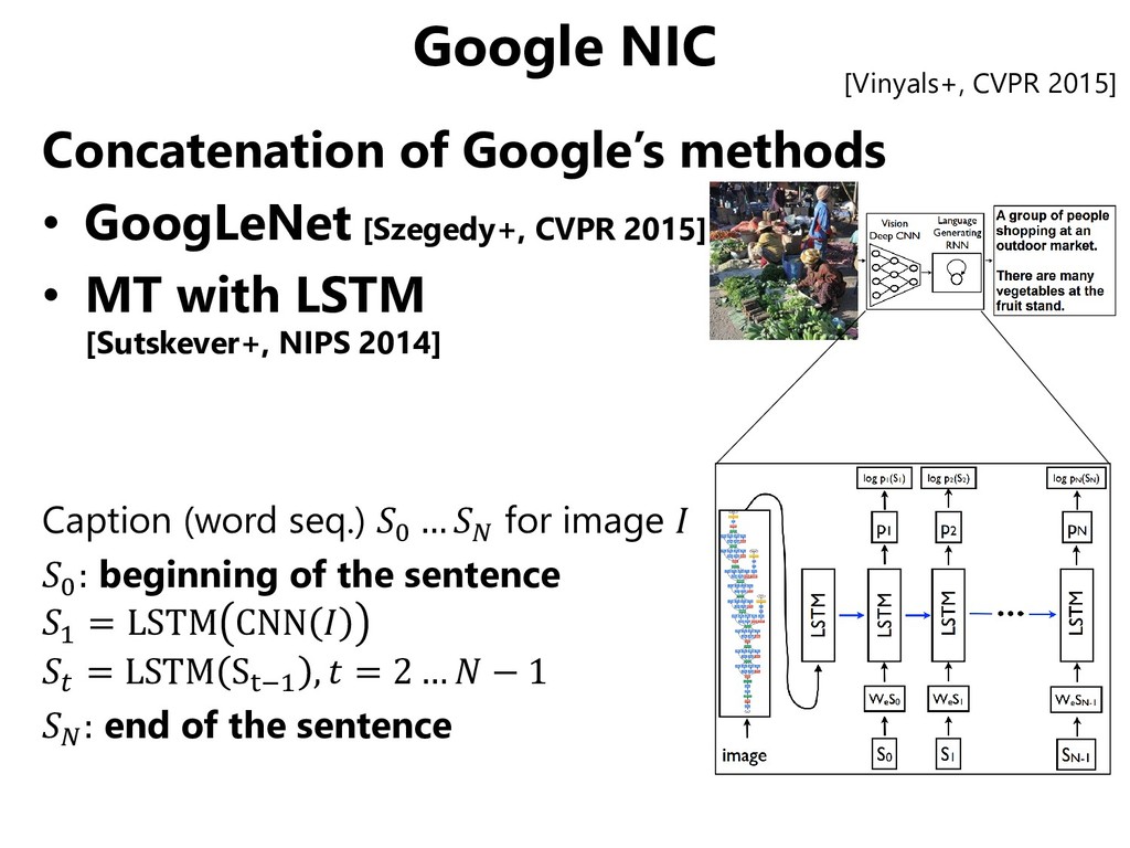
in machine translation [Sutskever+, NIPS 2014] – LSTM [Hochreiter+Schmidhuber, 1997] solves the gradient vanishing problem in RNN →Dealing with relations between distant words in a sentence – Four-layer LSTM is trained in an end-to-end manner →comparable to state-of-the-art (English to French) • Emergence of common techs such as CNN/RNN Reduction of barriers to get into CV+NLP Input Output
• Facebook: 300 million photos per day • YouTube: 400-hours videos per minute Pōhutukawa blooms this time of the year in New Zealand. As the flowers fall, the ground underneath the trees look spectacular. Pairs of a sentence + a video / photo →Collectable in large quantities
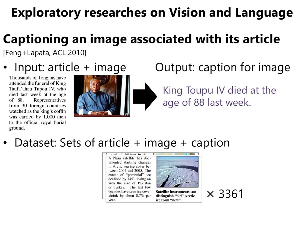
with its article [Feng+Lapata, ACL 2010] • Input: article + image Output: caption for image • Dataset: Sets of article + image + caption × 3361 King Toupu IV died at the age of 88 last week.
with its article [Feng+Lapata, ACL 2010] • Input: article + image Output: caption for image • Dataset: Sets of article + image + caption × 3361 King Toupu IV died at the age of 88 last week. As a result of these backgrounds: Various research topics such as …
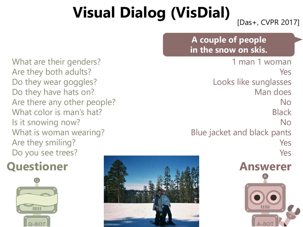
the snow on skis. What are their genders? Are they both adults? Do they wear goggles? Do they have hats on? Are there any other people? What color is man’s hat? Is it snowing now? What is woman wearing? Are they smiling? Do you see trees? 1 man 1 woman Yes Looks like sunglasses Man does No Black No Blue jacket and black pants Yes Yes [Das+, CVPR 2017]
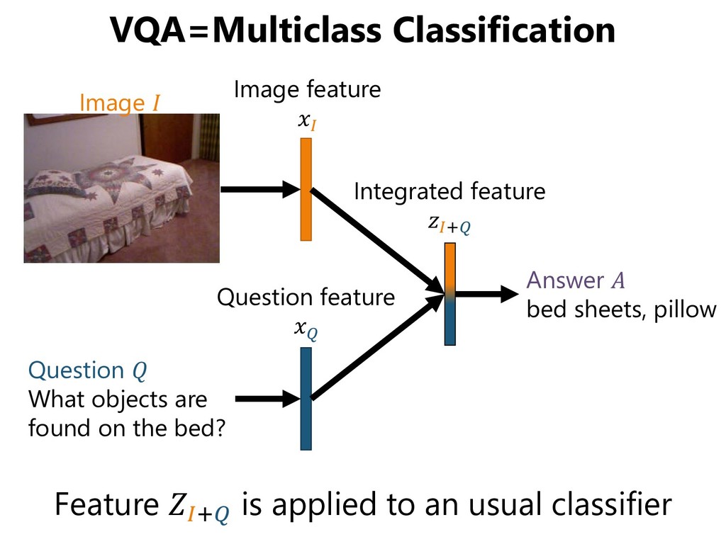
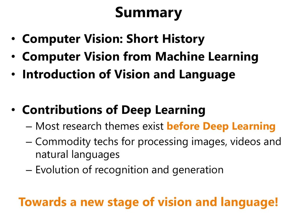
Machine Learning • Introduction of Vision and Language • Contributions of Deep Learning – Most research themes exist before Deep Learning – Commodity techs for processing images, videos and natural languages – Evolution of recognition and generation Towards a new stage of vision and language!
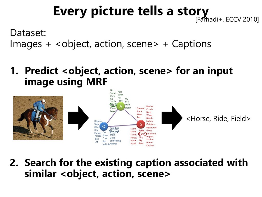
scene> + Captions 1. Predict <object, action, scene> for an input image using MRF 2. Search for the existing caption associated with similar <object, action, scene> <Horse, Ride, Field> [Farhadi+, ECCV 2010]
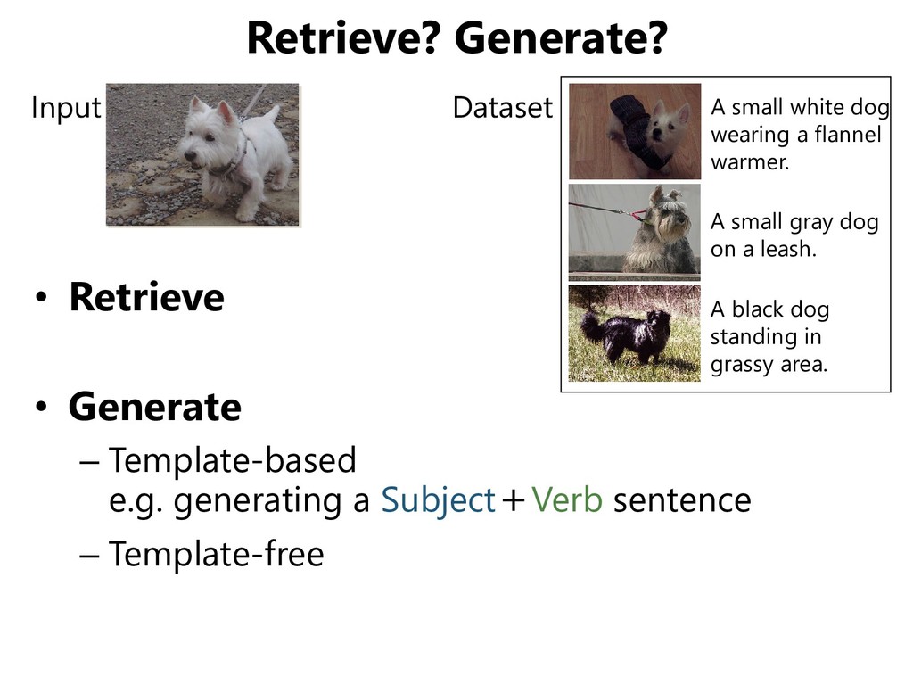
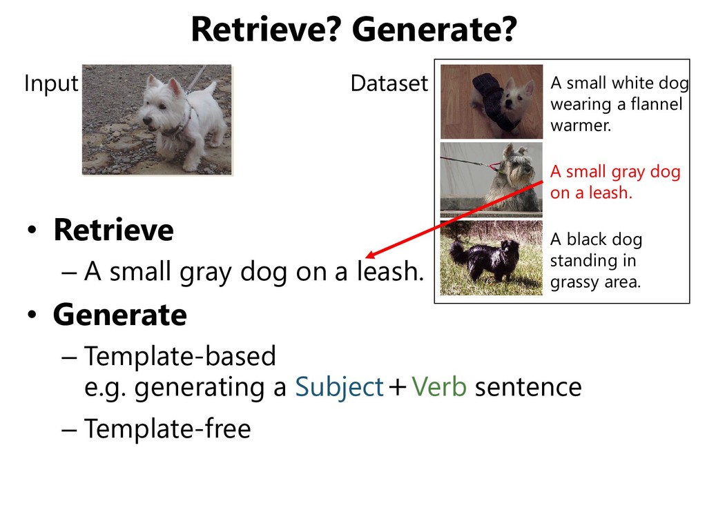
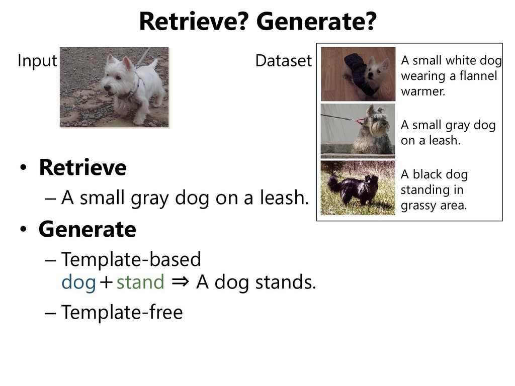
a Subject+Verb sentence – Template-free A small gray dog on a leash. A black dog standing in grassy area. A small white dog wearing a flannel warmer. Input Dataset
a leash. • Generate – Template-based e.g. generating a Subject+Verb sentence – Template-free A small gray dog on a leash. A black dog standing in grassy area. A small white dog wearing a flannel warmer. Input Dataset
a leash. • Generate – Template-based dog+stand ⇒ A dog stands. – Template-free A small gray dog on a leash. A black dog standing in grassy area. A small white dog wearing a flannel warmer. Input Dataset
a leash. • Generate – Template-based dog+stand ⇒ A dog stands. – Template-free A small white dog standing on a leash. A small gray dog on a leash. A black dog standing in grassy area. A small white dog wearing a flannel warmer. Input Dataset
NIPS 2012] • Deep learning appears in machine translation [Sutskever+, NIPS 2014] – LSTM [Hochreiter+Schmidhuber, 1997] solves the gradient vanishing problem in RNN →Dealing with relations between distant words in a sentence – Four-layer LSTM is trained in an end-to-end manner →comparable to state-of-the-art (English to French) Emergence of common techs such as CNN/RNN Reduction of barriers to get into CV+NLP Input Output
MM 2012]: Conventional object recognition Fisher Vector + Linear classifier Neural image captioning: Conventional object recognition Convolutional Neural Network Neural image captioning Conventional machine translation Recurrent Neural Network + beam search [Ushiku+, ACM MM 2012]: Conventional machine translation Log Linear Model + beam search Estimation of important words Connect the words with grammar model • Trained using only images and captions • Approaches are similar to each other
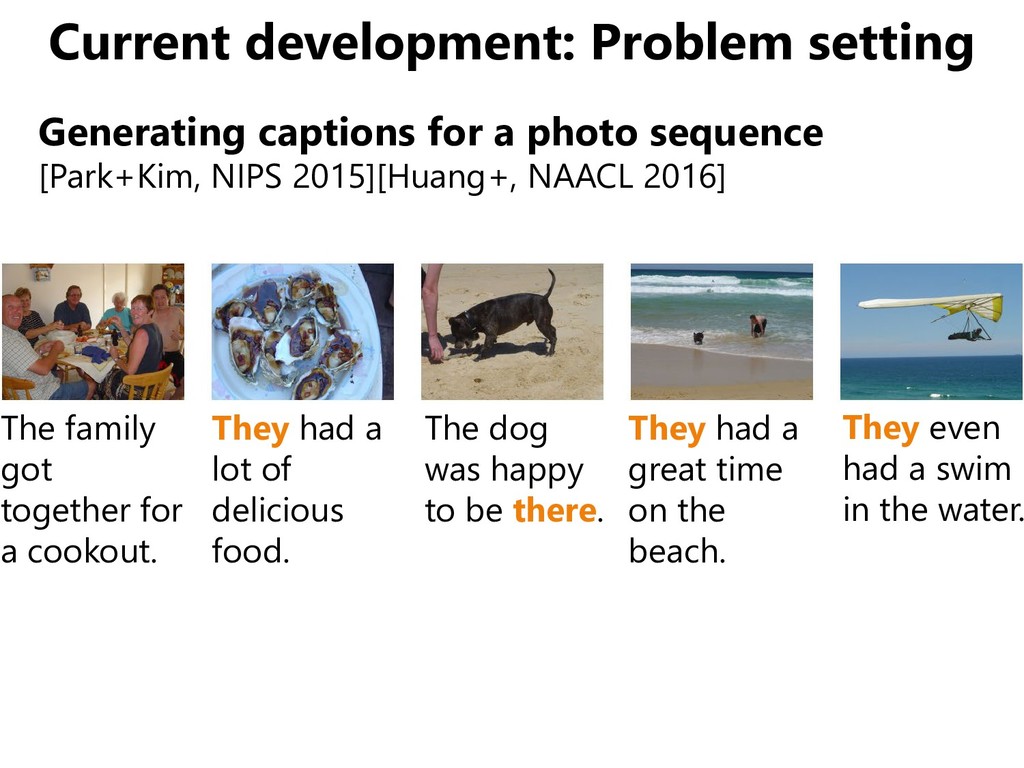
[Park+Kim, NIPS 2015][Huang+, NAACL 2016] The family got together for a cookout. They had a lot of delicious food. The dog was happy to be there. They had a great time on the beach. They even had a swim in the water.
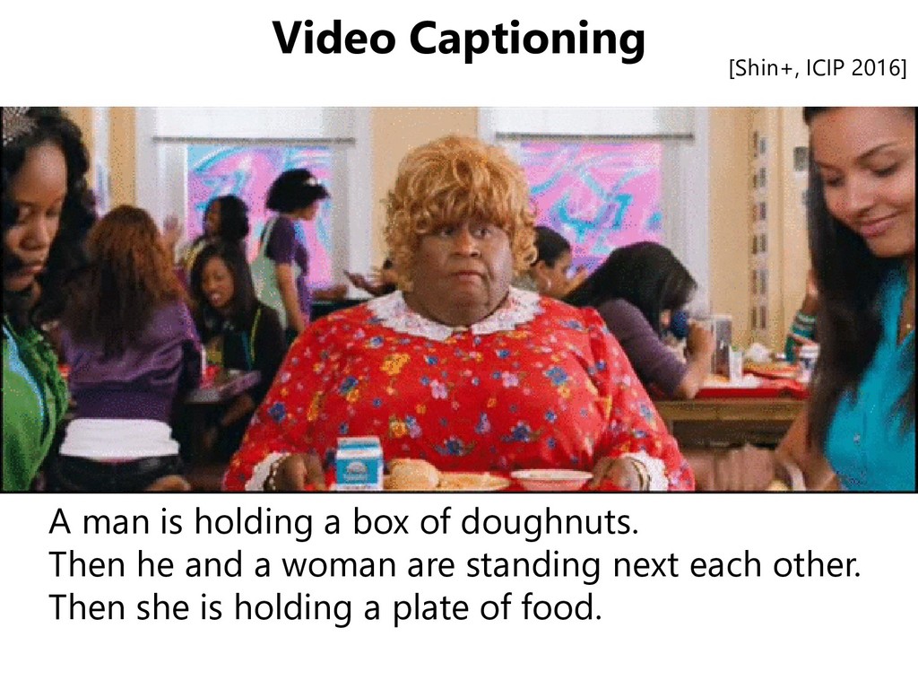
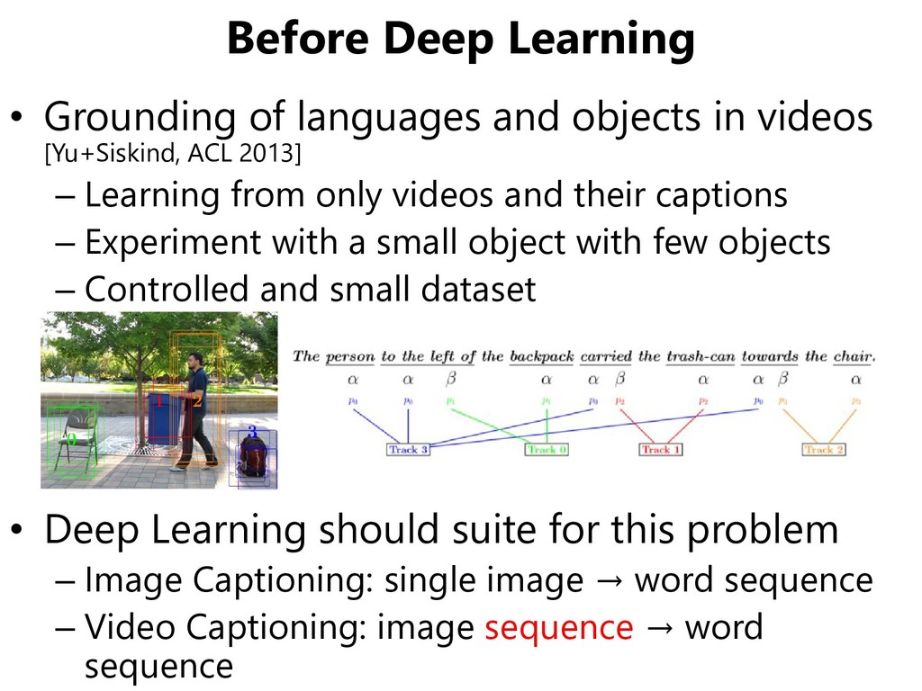
videos [Yu+Siskind, ACL 2013] – Learning from only videos and their captions – Experiment with a small object with few objects – Controlled and small dataset • Deep Learning should suite for this problem – Image Captioning: single image → word sequence – Video Captioning: image sequence → word sequence
– CNN+RNN for • Action recognition • Image / Video Captioning • Video to Text [Venugopalan+, ICCV 2015] – CNNs to recognize • Objects from RGB frames • Actions from flow images – RNN for captioning
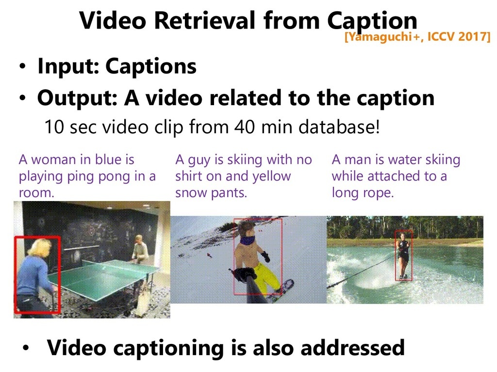
video related to the caption 10 sec video clip from 40 min database! • Video captioning is also addressed A woman in blue is playing ping pong in a room. A guy is skiing with no shirt on and yellow snow pants. A man is water skiing while attached to a long rope. [Yamaguchi+, ICCV 2017]
![VGGNet and Inception • VGGNet[Simonyan+Zisserman, ICLR 2015] – CNN desined](https://files.speakerdeck.com/presentations/78d60044a3f943d5b6f04e9fa0add5bc/slide_24.jpg)
![Object Detection • RCNN (Region CNN) [Girshick+, CVPR 2014] –](https://files.speakerdeck.com/presentations/78d60044a3f943d5b6f04e9fa0add5bc/slide_26.jpg)
![Semantic Segmentation • U-Net [Ronneberger+, MICCAI 2015] – Autoencoder +](https://files.speakerdeck.com/presentations/78d60044a3f943d5b6f04e9fa0add5bc/slide_27.jpg)
![From 2D to 3D: PointNet [Qi+, CVPR 2017]](https://files.speakerdeck.com/presentations/78d60044a3f943d5b6f04e9fa0add5bc/slide_28.jpg)
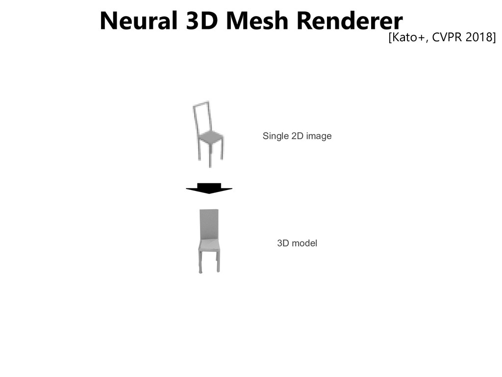
![Neural 3D Mesh Renderer [Kato+, CVPR 2018]](https://files.speakerdeck.com/presentations/78d60044a3f943d5b6f04e9fa0add5bc/slide_29.jpg)
![UDA by Pseudo-Labeling [Saito+, ICML 2017]](https://files.speakerdeck.com/presentations/78d60044a3f943d5b6f04e9fa0add5bc/slide_35.jpg)
![Maximum Classifier Discrepancy (MCD) [Saito+, CVPR 2018]](https://files.speakerdeck.com/presentations/78d60044a3f943d5b6f04e9fa0add5bc/slide_62.jpg)
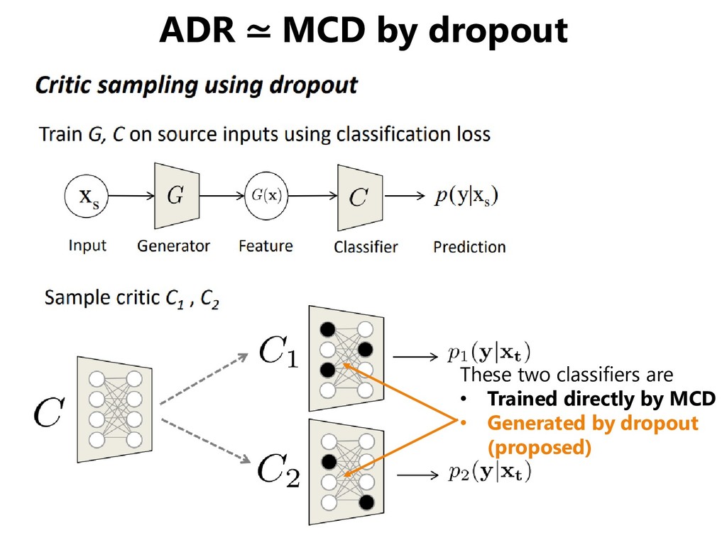
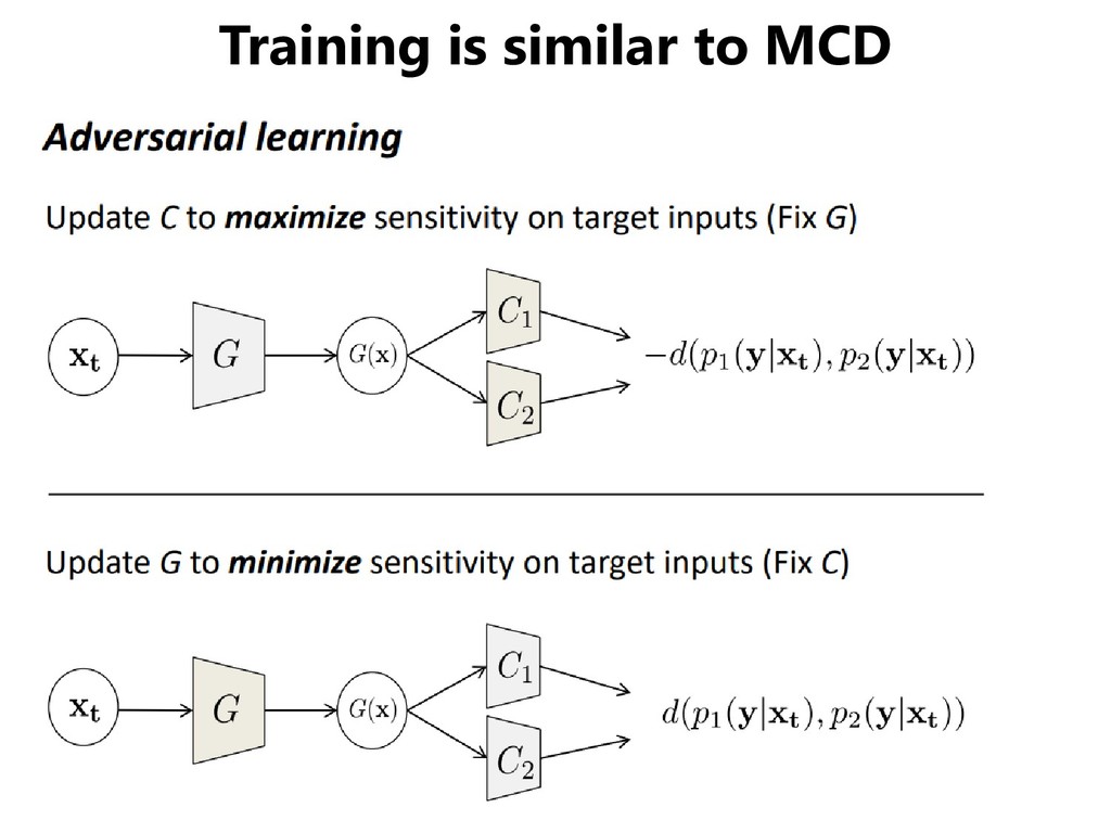
![Adversarial Dropout Regularization (ADR) [Saito+, ICLR 2018]](https://files.speakerdeck.com/presentations/78d60044a3f943d5b6f04e9fa0add5bc/slide_71.jpg)
![Open Set Domain Adaptation (OSDA) [Saito+, ECCV 2018]](https://files.speakerdeck.com/presentations/78d60044a3f943d5b6f04e9fa0add5bc/slide_77.jpg)
![OSDA by Backpropagation [Saito+, ECCV 2018]](https://files.speakerdeck.com/presentations/78d60044a3f943d5b6f04e9fa0add5bc/slide_79.jpg)
![Domain Adaptation for Object Detection [Saito+, CVPR 2019]](https://files.speakerdeck.com/presentations/78d60044a3f943d5b6f04e9fa0add5bc/slide_80.jpg)
![Strong-Weak Distribution Alignment [Saito+, CVPR 2019]](https://files.speakerdeck.com/presentations/78d60044a3f943d5b6f04e9fa0add5bc/slide_81.jpg)
![Image Captioning [Ushiku+, ACM Multimedia 2012]](https://files.speakerdeck.com/presentations/78d60044a3f943d5b6f04e9fa0add5bc/slide_87.jpg)
![Image Captioning [Ushiku+, ACM Multimedia 2012]](https://files.speakerdeck.com/presentations/78d60044a3f943d5b6f04e9fa0add5bc/slide_88.jpg)
![Multilingual Captioning Transfer learning among languages [Miyazaki+Shimizu, ACL 2016] •](https://files.speakerdeck.com/presentations/78d60044a3f943d5b6f04e9fa0add5bc/slide_91.jpg)
![Visual Question Answering [Fukui+, EMNLP 2016]](https://files.speakerdeck.com/presentations/78d60044a3f943d5b6f04e9fa0add5bc/slide_93.jpg)
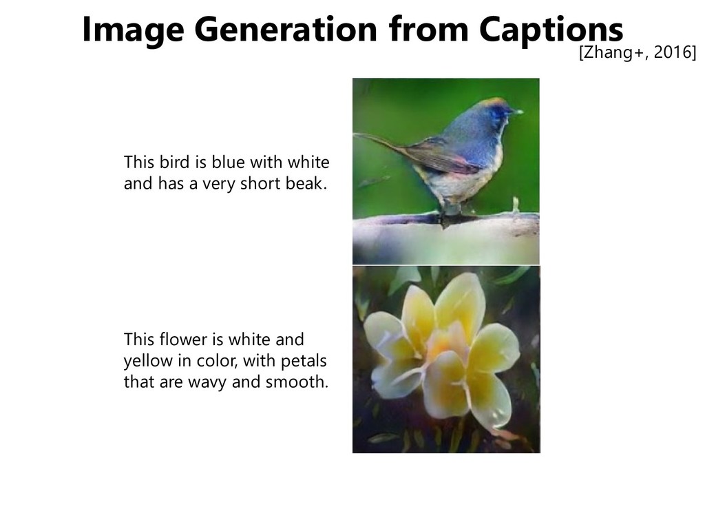
![Towards more realistic image generation StackGAN [Zhang+, 2016] Two-step GANs](https://files.speakerdeck.com/presentations/78d60044a3f943d5b6f04e9fa0add5bc/slide_96.jpg)
![Vision-and-Language Navigation (VNL) [Anderson+, ICCV 2017]](https://files.speakerdeck.com/presentations/78d60044a3f943d5b6f04e9fa0add5bc/slide_99.jpg)
![Captioning with multi-keyphrases [Ushiku+, ACM MM 2012]](https://files.speakerdeck.com/presentations/78d60044a3f943d5b6f04e9fa0add5bc/slide_109.jpg)
![End of sentence [Ushiku+, ACM MM 2012]](https://files.speakerdeck.com/presentations/78d60044a3f943d5b6f04e9fa0add5bc/slide_110.jpg)
![Examples of generated captions [https://github.com/tensorflow/models/tree/master/im2txt] [Vinyals+, CVPR 2015]](https://files.speakerdeck.com/presentations/78d60044a3f943d5b6f04e9fa0add5bc/slide_113.jpg)
![Comparison to [Ushiku+, ACM MM 2012] Input image [Ushiku+, ACM](https://files.speakerdeck.com/presentations/78d60044a3f943d5b6f04e9fa0add5bc/slide_114.jpg)
![Current development: Accuracy • Attention-based captioning [Xu+, ICML 2015] –](https://files.speakerdeck.com/presentations/78d60044a3f943d5b6f04e9fa0add5bc/slide_115.jpg)
![Current development: Problem setting Dense captioning [Lin+, BMVC 2015] [Johnson+,](https://files.speakerdeck.com/presentations/78d60044a3f943d5b6f04e9fa0add5bc/slide_116.jpg)
![End-to-end learning by Deep Learning • LRCN [Donahue+, CVPR 2015]](https://files.speakerdeck.com/presentations/78d60044a3f943d5b6f04e9fa0add5bc/slide_120.jpg)