Develop Numerical Software (PyConTW 2019)

Numerical software development is a unique subject. On one hand, programming skills and computer science are indispensable for proper implementation. On the other hand, the understandings to the scientific or engineering problems are the foundation of the software. The fundamental knowledge is so important that the application experts, e.g., mathematicians and scientists, often become the best programmers. However, it is difficult to train people for the multi-disciplinary skills. This talk will discuss how Python makes the development and training manageable.

HackMD: https://hackmd.io/@PyConTW/2019/%2F%40pycontw%2FrJMLHj2UH

Transcript

1. Develop Numerical Software Yung-Yu Chen
 yyc@solvcon.net PyCon Taiwan, 21st September 2019 1
2. Problems to solve • Mathematics • Statistics • Data analytics • Geometry • Physics • Particle physics • Quantum mechanics • Astrophysics • Engineering • Mechanics • Finite-difference, finite- element, finite-volume • Heat transfer, fluid dynamics • Electromagnetic • Optics • And many others … !2
3. Numerical software • Research code • Useful codes are usually in clear-code • Niche markets • Merchandisable, but the user base is tiny • Usually too expensive for personal use • Long lifecycle, measured by decade, if surviving in the first place !3
4. Conservation-law solver • For example, my project is to make solvers that can simulate any physical processes governed by conservation laws:
 (three-dimensional system) ∂u ∂t + 3 ∑ k=1 A(k)(u) ∂u ∂xk = 0 j x 0 1 2 3 4 1 2 3 2 5 2 7 2 n t 0 1 2 1 Space-time stencil for the simplified one-dimensional system
 
 ∂u ∂t + ∂f(u) ∂x = 0 !4
5. got math? • , is the column vector of the solution variables, and is the Jacobian matrices of the flux functions. • We cannot innovate without knowing well about what we code for. • How practical it is to ask everyone to know well about it? ∂u ∂t + 3 ∑ k=1 A(k)(u) ∂u ∂xk = 0 u A(k)(u) !5
6. Engineering • We develop the numerical software for both science and engineering. We also need both science and “engineering” to develop the numerical software. • Tools and skills: • Python, numpy, and C++ • Code for high-performance: timing and latency • Memory management and diagnostics • Software engineering • System architecture • How to distribute and deploy open-source science code !6
7. Python, Numpy, C++ • In the good old days, numerical programmers speak Fortran, which is still the standard today. BLAS and LAPACK continue to use Fortran as the reference implementation. • Basic Linear Algebra Subprograms: http://www.netlib.org/blas/, defines the interface for vector, matrix-vector, and matrix-matrix operations. • Linear Algebra PACKage: http://www.netlib.org/lapack/, on top of BLAS, defines the interface for linear algebra toolboxes including linear solver, least square extrema finding, and eigenvalue and singular value problems. • Python is too slow for numerical calculation. (Pure Python is 100x slower than C for number-crunching.) But it’s so convenient to drive highly optimized computing kernels, with the help of Numpy. !7
8. Contiguous memory buffer • Numpy ndarray (N-dimensional array) is data structure describing a contiguous memory buffer • data: pointer to the memory buffer • nd: number of dimension • dimensions and strides: number of skips of elements and bytes in each dimension typedef struct { PyObject_HEAD PyTypeObject *typeobj; char kind; char type; char byteorder; char flags; int type_num; int elsize; int alignment; PyArray_ArrayDescr *subarray; PyObject *fields; PyObject *names; PyArray_ArrFuncs *f; PyObject *metadata; NpyAuxData *c_metadata; npy_hash_t hash; } PyArray_Descr; typedef struct PyArrayObject { PyObject_HEAD char *data; int nd; npy_intp *dimensions; npy_intp *strides; PyObject *base; PyArray_Descr *descr; int flags; PyObject *weakreflist; } PyArrayObject; !8
9. Crunch real numbers • Example: solve the Laplace equation • • • • Double-precision is commonplace • Point-Jacobi method: 3-level nested loop ∂2u ∂x2 + ∂2u ∂y2 = 0 (0 < x < 1; 0 < y < 1) u(0,y) = 0, u(1,y) = sin(πy) (0 ≤ y ≤ 1) u(x,0) = 0, u(x,1) = 0 (0 ≤ x ≤ 1) def solve_python_loop(): u = uoriginal.copy() un = u.copy() converged = False step = 0 # Outer loop. while not converged: step += 1 # Inner loops. One for x and the other for y. for it in range(1, nx-1): for jt in range(1, nx-1): un[it,jt] = (u[it+1,jt] + u[it-1,jt] + u[it,jt+1] + u[it,jt-1]) / 4 norm = np.abs(un-u).max() u[...] = un[...] converged = True if norm < 1.e-5 else False return u, step, norm !9
10. Power of Numpy def solve_array(): u = uoriginal.copy() un = u.copy() converged = False step = 0 while not converged: step += 1 un[1:nx-1,1:nx-1] = (u[2:nx,1:nx-1] + u[0:nx-2,1:nx-1] + u[1:nx-1,2:nx] + u[1:nx-1,0:nx-2]) / 4 norm = np.abs(un-u).max() u[...] = un[...] converged = True if norm < 1.e-5 else False return u, step, norm def solve_python_loop(): u = uoriginal.copy() un = u.copy() converged = False step = 0 # Outer loop. while not converged: step += 1 # Inner loops. One for x and the other for y. for it in range(1, nx-1): for jt in range(1, nx-1): un[it,jt] = (u[it+1,jt] + u[it-1,jt] + u[it,jt+1] + u[it,jt-1]) / 4 norm = np.abs(un-u).max() u[...] = un[...] converged = True if norm < 1.e-5 else False return u, step, norm CPU times: user 57.9 ms, sys: 1.43 ms, total: 59.3 ms Wall time: 58.3 ms CPU times: user 5.2 s, sys: 19.5 ms, total: 5.22 s Wall time: 5.24 s 5.24 s (pure Python) / 58.3 ms (Numpy) = 89.88 x !10
11. Multi-dimensional arrays • Numpy ndarray allows easy manipulation of multi-dimensional arrays (2D arrays for matrices). • Take an matrix for example. We expect to access its elements with a[i,j], where i is the row index, and j the column index. • The mathematical layout of the array. • The physical layout in computer • Higher dimensional arrays work the same way m × n m × n a11 a12 a1n ⋯ a21 a22 a2n ⋯ ⋮ ⋮ ⋱ am1 am2 amn ⋯ a11 a12 ⋯ a1n a21 ⋯ am1 ⋯ amn ← contiguous in memory !11
12. Create multi-dimensional arrays • Stack vertically to create the second dimension
 
 
 
 
 
 
 • Be careful about majoring ranged_array = np.arange(10) print("A 1D array:", ranged_array) A 1D array: [0 1 2 3 4 5 6 7 8 9] hstack_array = np.hstack([ranged_array, ranged_array]) print("Horizontally stacked array:", hstack_array) Horizontally stacked array: [0 1 2 3 4 5 6 7 8 9 0 1 2 3 4 5 6 7 8 9] vstack_array = np.vstack([ranged_array, ranged_array]) print("Vertically stacked array:", vstack_array) Vertically stacked array: [[0 1 2 3 4 5 6 7 8 9] [0 1 2 3 4 5 6 7 8 9]] original_array = np.arange(6) print("original 1D array:", original_array) original 1D array: [0 1 2 3 4 5] print("reshaped 2D array:", original_array.reshape((2,3))) reshaped 2D array: [[0 1 2] [3 4 5]] print("reshaped 2D array:", original_array.reshape((2,3), order='f')) reshaped 2D array: [[0 2 4] [1 3 5]] ← row major: last index changes the fastest (default) ← column major: first index changes the fastest !12
13. Zero-copy: do it where it fits Python app C++ app C++ container Ndarray manage access Python app C++ app C++ container Ndarray manage access a11 a12 ⋯ a1n a21 ⋯ am1 ⋯ amn a11 a12 ⋯ a1n a21 ⋯ am1 ⋯ amn memory buffer shared across language memory buffer shared across language Top (Python) - down (C++) Bottom (C++) - up (Python) Python app C++ app a11 a12 ⋯ a1n a21 ⋯ am1 ⋯ amn memory buffer shared across language Ndarray C++ container !13
14. High-performance code • The number-crunching code is in deep or long loops. It’s the calculation kernel that we try to optimize as much as possible. • Other code is considered “house-keeping”. It’s equally important, and where we architect. • Our job is is to keep the calculation kernel compact and optimize it as much as we can. !14
15. Timing for hotspots • Do not optimize code right away! • We can’t afford to optimize everything • We need to time everywhere to find hotspots • Plan for timing from the beginning !15 The first principle is that you must not fool yourself and you are the easiest person to fool. — Richard P. Feynman
16. Types of time • CPU time: measure the number of clocks spent in CPU cores • User time: spent in the user code • System time: spent in the OS • Wall time: the time duration in real world (clock on the wall) • CPU time can be bigger than wall time cpu1 5 sec 5 sec 20 sec cpu2 20 sec 30 sec !16
17. Time the whole executable • Linux time command: • real: the wall time • user: user time (CPU) • sys: system time (CPU) $ time ls > /dev/null real 0m0.011s user 0m0.002s sys 0m0.008s !17
18. Make your own stopwatch • Automatic tools fall short when we need special granularity • Python timer for prototype and high-level operations • timeit module times Python one-liners. By default it measures the wall time.
 
 • time module provides detailed timing API: perf_counter(), perf_counter_ns() • Linux timer for low-level oprations • CPU clock timer:
 • Wall timer: $ python3 -m timeit '"-".join(str(n) for n in range(100))' 10000 loops, best of 5: 22.8 usec per loop clock_t times (struct tms *buffer); int gettimeofday (struct timeval *tp, struct timezone *tzp); !18
19. Memory hierarchy • Modern computer has faster CPU than memory • High performance comes with hiding the latency registers (0 cycle) L1 cache (4 cycles) L2 cache (10 cycles) L3 cache (50 cycles) Main memory (200 cycles) Disk (storage) (100,000 cycles) !19
20. Locality CPU a11 a12 ⋯ a1n a21 ⋯ am1 ⋯ amn 1st read (200 cycles) 2nd read (200 cycles) CPU a11 a12 ⋯ a1n a21 ⋯ am1 ⋯ amn 1st read (200 cycles) 2nd read (4 cycles) Bad spatial locality:
 200 + 200 = 400 cycles Cached by 1st read Cached by 1st read Good spatial locality:
 200 + 4 = 204 cycles Cache miss: 200 cycles
 Cache hit: 4 cycles !20
21. Locality, cont’d • Test how it works using matrix-vector multiplication: • Numpy by default uses row-major • Column-major is slower than row- major (2.3 times) • double is faster than int64! y = Ax mat_rmajor = np.arange(100000000, dtype='float64').reshape((10000,10000)) mat_cmajor = mat_rmajor.T.copy().T vec = np.arange(10000, dtype='float64') %%time res_rmajor = np.dot(mat_rmajor, vec) CPU times: user 58.6 ms, sys: 1.46 ms, total: 60.1 ms Wall time: 59.2 ms %%time res_cmajor = np.dot(mat_cmajor, vec) CPU times: user 134 ms, sys: 2.21 ms, total: 136 ms Wall time: 136 ms mat_rmajor = np.arange(100000000, dtype='int64').reshape((10000,10000)) mat_cmajor = mat_rmajor.T.copy().T vec = np.arange(10000, dtype='int64') %%time res_rmajor = np.dot(mat_rmajor, vec) CPU times: user 69.7 ms, sys: 1.22 ms, total: 70.9 ms Wall time: 69.7 ms %%time res_cmajor = np.dot(mat_cmajor, vec) CPU times: user 802 ms, sys: 1.85 ms, total: 804 ms Wall time: 802 ms ↑ With Mac or anaconda, you may get more interesting results than above ↑ !21
22. Memory management • Profile for memory is much more difficult than for runtime • You need your own malloc, realloc, calloc, and free, and C++ Allocator template, which has to be done in C/C++ • It’s the last resort, but last resort is usually needed for industry-grade code • However, it’s common for a system to start with simple Python prototype, which of course doesn’t do any of above • Architecture based on Python objects usually doesn’t scale, think twice before doing that !22
23. Large memory • The number-crunching kernel usually allocates big chunks of memory, rather than small pieces • matrix of double-precision takes 800 MB • Other common data: mesh (grid), field, indices, etc. • Zero-copy applies here • Huge pages are useful 10,000 × 10,000 !23
24. Instance counting template <class T> class InstanceCounter { public: InstanceCounter() { ++m_constructed; } InstanceCounter(InstanceCounter const & other) { ++m_constructed; } ~InstanceCounter() { ++m_destructed; } static std::size_t active() { return m_constructed - m_destructed; } static std::size_t constructed() { return m_constructed; } static std::size_t destructed() { return m_destructed; } private: static std::atomic_size_t m_constructed; static std::atomic_size_t m_destructed; }; /* end class InstanceCounter */ template <class T> std::atomic_size_t InstanceCounter<T>::m_constructed = 0; template <class T> std::atomic_size_t InstanceCounter<T>::m_destructed = 0; !24
25. Memory tips • When modularizing the code, put a memory manager in each module • Know what module uses how much memory • Special treatment when necessary • Very difficult to insert the manager layer afterwards • Allow the system to switch between different global memory managers: glibc, jemalloc, tcmalloc, etc. • Use runtime analyzers like valgrind • Learn PyMem !25
26. Software engineering • Keyword: automation • Human makes mistakes, programmers make more, which are called bugs • Version control is the foundation • Critical parts: • Build system • Unit testing • Code review !26
27. Build system • Makefile (GNU make) is our good friend • It’s old but concise and well documented; useable as long as you have bash • Use cmake when project grows • It's cross-platform and works well with IDE • You may still use Python distutils, but it’s not convenient for intensive C++ code and dependency !27
28. GNU make • Define variables • Define rules, which include the recipe (commands to run) CXX = g++ hello: hello.o hellomain.o $(CXX) hello.o hellomain.o -o hello hello.o: hello.cpp hello.hpp $(CXX) -c hello.cpp -o hello.o hellomain.o: hellomain.cpp hello.hpp $(CXX) -c hellomain.cpp -o hellomain.o !28
29. Unit testing • Google-test for C++ • Python stdlib unittest and py.test • Some C++ things can only be tested with Google-test, like template • C++ code doesn’t need to be tested exclusively with Google-test • Non-template code can be wrapped to Python for testing • Help both convenience and quality !29
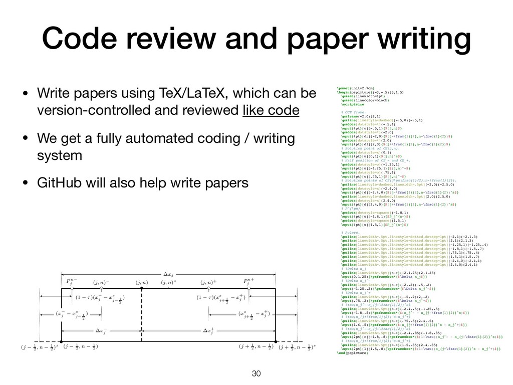
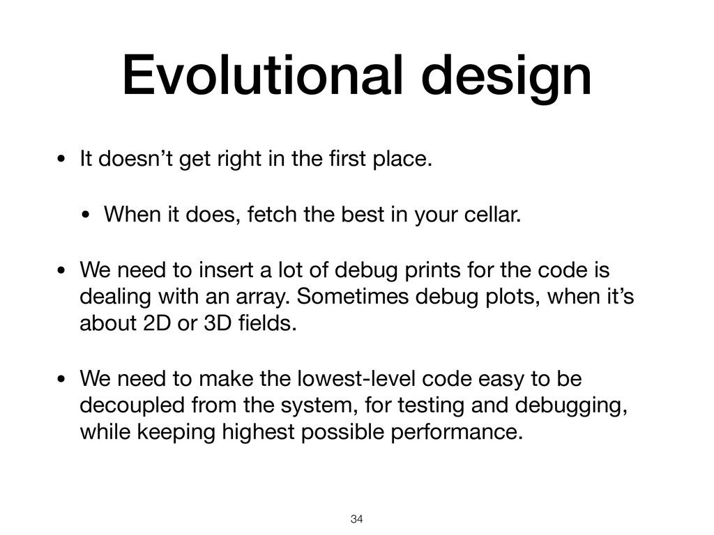
30. Code review and paper writing • Write papers using TeX/LaTeX, which can be version-controlled and reviewed like code • We get a fully automated coding / writing system • GitHub will also help write papers !30 \psset{unit=2.7cm} \begin{pspicture}(-3,-.5)(3,1.5) \psset{linewidth=1pt} \psset{linecolor=black} \scriptsize % CCE frame. \psframe(-2,0)(2,1) \psline[linestyle=dashed](-.5,0)(-.5,1) \psdots[dotstyle=*](-.5,1) \uput{4pt}[u](-.5,1){$(j,n)$} \psdots[dotstyle=*](-2,0) \uput{4pt}[dr](-2,0){$(j-\frac{1}{2},n-\frac{1}{2})$} \psdots[dotstyle=*](2,0) \uput{4pt}[dl](2,0){$(j+\frac{1}{2},n-\frac{1}{2})$} % Solution point of CE(j,n). \psdots[dotstyle=x](0,1) \uput{4pt}[u](0,1){$(j,n)^s$} % Half position of CE_- and CE_+. \psdots[dotstyle=o](-1.25,1) \uput{4pt}[u](-1.25,1){$(j,n)^-$} \psdots[dotstyle=o](.75,1) \uput{4pt}[u](.75,1){$(j,n)^+$} % Solution points of CE(j\pm\frac{1}{2},n-\frac{1}{2}). \psline[linestyle=dashed,linewidth=.5pt](-2,0)(-2.5,0) \psdots[dotstyle=x](-2.4,0) \uput{4pt}[d](-2.4,0){$(j-\frac{1}{2},n-\frac{1}{2})^s$} \psline[linestyle=dashed,linewidth=.5pt](2,0)(2.5,0) \psdots[dotstyle=x](2.4,0) \uput{4pt}[d](2.4,0){$(j+\frac{1}{2},n-\frac{1}{2})^s$} % P^{\pm}. \psdots[dotstyle=square](-1.8,1) \uput{4pt}[u](-1.8,1){$P_j^{n-}$} \psdots[dotstyle=square](1.5,1) \uput{4pt}[u](1.5,1){$P_j^{n+}$} % Rulers. \psline[linewidth=.5pt,linestyle=dotted,dotsep=1pt](-2,1)(-2,1.3) \psline[linewidth=.5pt,linestyle=dotted,dotsep=1pt](2,1)(2,1.3) \psline[linewidth=.5pt,linestyle=dotted,dotsep=1pt](-1.25,1)(-1.25,.4) \psline[linewidth=.5pt,linestyle=dotted,dotsep=1pt](-1.8,1)(-1.8,.7) \psline[linewidth=.5pt,linestyle=dotted,dotsep=1pt](.75,1)(.75,.4) \psline[linewidth=.5pt,linestyle=dotted,dotsep=1pt](1.5,1)(1.5,.7) \psline[linewidth=.5pt,linestyle=dotted,dotsep=1pt](-2.4,0)(-2.4,1) \psline[linewidth=.5pt,linestyle=dotted,dotsep=1pt](2.4,0)(2.4,1) % \Delta x_j \psline[linewidth=.5pt]{<->}(-2,1.25)(2,1.25) \rput(0,1.25){\psframebox*{$\Delta x_j$}} % \Delta x_j^- \psline[linewidth=.5pt]{<->}(-2,.2)(-.5,.2) \rput(-1.25,.2){\psframebox*{$\Delta x_j^-$}} % \Delta x_j^+ \psline[linewidth=.5pt]{<->}(-.5,.2)(2,.2) \rput(.75,.2){\psframebox*{$\Delta x_j^+$}} % \tau(x_j^--x_{j-\frac{1}{2})^s} \psline[linewidth=.5pt]{<->}(-2.4,.5)(-1.25,.5) \rput(-1.8,.5){\psframebox*{$(x_j^- - x_{j-\frac{1}{2}}^s)$}} % \tau(x_{j+\frac{1}{2})^s-x_j^+} \psline[linewidth=.5pt]{<->}(.75,.5)(2.4,.5) \rput(1.6,.5){\psframebox*{$(x_{j+\frac{1}{2}}^s - x_j^+)$}} % \tau(x_j^--x_{j-\frac{1}{2})^s} \psline[linewidth=.5pt]{<->}(-2.4,.85)(-1.8,.85) \uput{2pt}[r](-1.8,.8){\psframebox*{$(1-\tau)(x_j^- - x_{j-\frac{1}{2}}^s)$}} % \tau(x_{j+\frac{1}{2})^s-x_j^+} \psline[linewidth=.5pt]{<->}(1.5,.85)(2.4,.85) \uput{2pt}[l](1.5,.8){\psframebox*{$(1-\tau)(x_{j+\frac{1}{2}}^s - x_j^+)$}} \end{pspicture} (j, n) (j − 1 2 , n − 1 2 ) (j + 1 2 , n − 1 2 ) · (j, n)s (j, n)− (j, n)+ · (j − 1 2 , n − 1 2 )s · (j + 1 2 , n − 1 2 )s P n− j P n+ j ∆xj ∆x− j ∆x+ j (x− j − xs j− 1 2 ) (xs j+ 1 2 − x+ j ) (1 − τ)(x− j − xs j− 1 2 ) (1 − τ)(xs j+ 1 2 − x+ j )
31. System design patterns • Goals: • Data parallel • Object-orientation • Scriptability • Design for testing • I/O and in situ processing !31
32. Data object • Numerical software processes huge amount of data. Copying them is expensive. • Use a pipeline to process the same block of data • Use an object to manage the data: data object • In other fields data objects may not always be a good idea. • Here, to get the best code structure with uncompromisable performance, we usually don’t find anything better than it. Field initialization Interior time-marching Boundary condition Parallel data sync Finalization Data !32 Data access at all phases
33. Nested loop • Nested loops are everywhere in numerical methods • They are also in linear algebra code • Except in high-level flow control, there’s no room for fancy things like list comprehension or generator def solve_python_loop(): u = uoriginal.copy() un = u.copy() converged = False step = 0 # Outer loop. while not converged: step += 1 # Inner loops. One for x and the other for y. for it in range(1, nx-1): for jt in range(1, nx-1): un[it,jt] = (u[it+1,jt] + u[it-1,jt] + u[it,jt+1] + u[it,jt-1]) / 4 norm = np.abs(un-u).max() u[...] = un[...] converged = True if norm < 1.e-5 else False return u, step, norm Point Jacobi → !33
34. Evolutional design • It doesn’t get right in the first place. • When it does, fetch the best in your cellar. • We need to insert a lot of debug prints for the code is dealing with an array. Sometimes debug plots, when it’s about 2D or 3D fields. • We need to make the lowest-level code easy to be decoupled from the system, for testing and debugging, while keeping highest possible performance. !34
35. Release and distribution • Research code may be distributed in a source form: git clone • “Users” of a research code are like high-level developers, sometimes dig into the details as they need • Research code should be properly engineered in the beginning • If not, during productization it will be rewritten from ground up • When the code may be used in non-source form, consider packaging it for distribution • You may also need packaging when open source isn’t an option !35
36. PyPI • The Python Package Index (https://pypi.org/) is a repository of software for the Python programming language • Work best for pure Python code • Package using distutils (https://docs.python.org/3/ library/distutils.html) or setuptools (https:// setuptools.readthedocs.io/en/latest/) • It’s possible to build binaries using distutils, but it’s far from a convenient tool !36
37. Conda and conda-forge • Numerical software has a lot of dependencies in Fortran, C, and C++. It’s much more convenient to use a general package manager. • Conda (https://docs.conda.io/en/latest/) is for any language, but developed in Python • The directives for building a package is called a recipe • Anaconda cloud (https://anaconda.org/about) is a hosting service for conda packages • Third-party may provide their own packages, e.g., https:// anaconda.org/intel/ • Conda-forge is a system maintaining community-contributed packaging recipes !37
38. Packaging completes development flow • Even for research code, packaging completes the development flow and help us find issues that are not spot during development • It’s the first step to move from research code to a software product !38
39. Ultimate form? • Numerical code incorporates so much knowledge. • Users often have an advanced degree other than CS. • It can hardly be as popular as other software. • In the beginning, scientists want it to “just work”. In the end, they want to change every bit for their crazy ideas. • Is the current tool chain sufficient for the demand? I think not. We have a long way to go. !39