2021 Computer Vision with CNN

Computer Vision
University of Pavia
deep learning on AWS with Amazon SageMaker

View Slide

Luca Bianchi
AWS Hero, passionate about
serverless and machine learning
Slide Title
github.com/aletheia
https://it.linkedin.com/in/lucabianchipavia
https://speakerdeck.com/aletheia
www.ai4devs.io
@bianchiluca

View Slide

• What is Deep Learning?

• Frameworks and tools

• Deep Learning for Computer Vision
Slide Title
• Setting up

• Our
f
irst neural network
• Solving Deep Learning

• Use cases
• PyTorch Lightning

• Amazon SageMaker Platform
• Transfer Learning

View Slide

Section 1

View Slide

What is Deep Learning?
Module 1
A (not so) theoretical introduction

View Slide

• An analysis of the history of technology shows that technological change is exponential, contrary to the
common- sense “intuitive linear” view.

• Technology growth throughout history has been exponential, it is not gonna stop until reaches a point where
innovation is happening at a seemingly-in
f
inite pace. Kurzweil called this event singularity.
The Law of Accelerated Growth
Why is happening now?
• After the singularity, something completely new will shape
our world.
 
Arti
f
icial Narrow Intelligence is evolving into Arti
f
icial
General Intelligence, then into Arti
f
icial Super Intelligence.

View Slide

• First deep learning attempts are almost 50
years old, but have been under utilized due
to computing power constraints

• Datasets were too small to allow e
ff
icient
training of algorithms

• Some mathematical issues costrained the
adoption of powerful models (i.e. vanishing
gradients)
We’re at the nexus of converging opportunities
Why now?
Computing

Power
Huge dataset

availability
Backpropagation with
ReLU

View Slide

Wikipedia
“Arti
f
icial Intelligence

is the theory and development of computer systems able to perform tasks
normally requiring human intelligence, such as visual perception, speech
recognition, decision-making, and translation between languages.”

View Slide

Slide Title

View Slide

Slide Title
Symbolists
Use symbols,
rules, and logic
to represent
knowledge and
draw logical
inference
Favored
algorithm
Rules and
decision trees
Bayesians
Assess the
likelihood of
occurrence for
probabilistic
inference
Favored
algorithm
Naive Bayes or
Markov
Connectionists
Recognise and
generalise
patterns
dynamically
with matrices of
probabilistic
weighted
neurons
Favored
algorithm
Neural
Networks
Evolutionaries
Generate
variations and
then assess the
fi
tness of each
for a given
purpose
Favored
algorithm
Genetic
Programs
Analogizers
Optimize a
function in light
of constraints
(“going as high
as you can
while staying on
the road”)
Favored
algorithm
Support vectors
for decades individual “tribes” of
arti
fi
cial intelligence researchers
have vied one another for
dominance. Is the time now for
tribes to collaborate? They may
be forced to, as collaboration and
algorithm blending are the only
ways to reach true AGI.

View Slide

Slide Title

View Slide

Slide Title
The importance of Experience
• Machine Learning (ML) algorithms have data as input, ‘cause data represents the Experience. 
This is a focal point of Machine Learning: large amount of data is needed to achieve good performances.

• The Machine Learning equivalent of program in ML world is called ML model and improves over time as soon as
more data is provided, with a process called training.

• Data must be prepared (or
fi
ltered) to be suitable for training process. Generally input data must be collapsed into
a n-dimensional array with every item representing a sample.

• ML performances are measured in probabilistic terms, with metrics called accuracy or precision.
An operational de
fi
nition
“A computer program is said to learn from experience E with respect to some class of tasks T and performance
measure P if its performance at tasks in T, as measured by P, improves with experience E”

View Slide

Slide Title
Deterministic computing
Machine Learning
Computer
algorithm
data
output
Learner
data
output (e)
algorithm

View Slide

Slide Title
Input-based taxonomy
• Supervised Learning
• Unsupervised Learning
• Reinforcement Learning
Types of Machine Learning
Machine learning tasks are typically classi
fi
ed into three broad categories, depending on the nature of the learning
"signal" or "feedback" available to a learning system.
Output-based taxonomy
• Regression 
• Classi
fi
cation 
• Clustering 
• Density estimation 
• Dimensionality reduction

View Slide

“deep learning is a great phrase,

it seems so deep”

View Slide

Deep Learning
How “deep” is your deep learning?
• Deep Learning (DL) is based on non-linear structures that process information. The “deep” in name comes from
the contrast with “traditional” ML algorithms that usually use only one layer. What is a layer?

• A cost-function receiving data as input and outputting its function weights.

• More complex is the data you want to learn from, more layers are usually needed to learn from. The number of
layers is called depth of the DL algorithm.
An operational de
fi
nition
“A class of machine learning techniques that exploit many layers of non-linear information processing for supervised
or unsupervised feature extraction and transforma- tion, and for pattern analysis and classi
fi
cation.”

View Slide

Neural Networks
An operational de
fi
nition
“computing systems inspired by the biological neural networks that constitute animal brains. Such systems learn
(progressively improve performance) to do tasks by considering examples, generally without task-speci
fi
c programming”
An ANN is based on a collection of connected units called arti
fi
cial neurons, (analogous to axons in a biological brain).
Each connection (synapse) between neurons can transmit a signal to another neuron. The receiving (postsynaptic)
neuron can process the signal(s) and then signal downstream neurons connected to it. Neurons may have state,
generally represented by real numbers, typically between 0 and 1. Neurons and synapses may also have a weight that
varies as learning proceeds, which can increase or decrease the strength of the signal that it sends downstream.
Further, they may have a threshold such that only if the aggregate signal is below (or above) that level is the
downstream signal sent.

Typically, neurons are organized in layers. Di
ff
erent layers may perform di
ff
erent kinds of transformations on their inputs.
Signals travel from the
fi
rst (input), to the last (output) layer, possibly after traversing the layers multiple times.

View Slide

Anatomy of a Neural Network
A Perceptron A network of Perceptron

View Slide

Frameworks and tools
Module 2
How to build a neural network?

View Slide

Deep Learning Framework Landscape

View Slide

Framework landscape

View Slide

AWS Machine Learning stack

View Slide

Deep Learning

for Computer Vision
Module 3
Introduction to Convolutional Neural Networks

View Slide

Convolutional Neural Networks (ConvNets or CNNs) are a category of Neural Networks that have proven very effective
in areas such as image recognition and classification..

CNNs are based on Hierarchical Compositionality: we start from a low level input (pixel) and then we aggregate
informations up to an higher interpretation level.
A speci
f
ic kind of neural network

View Slide

Improved in just a few years
Revolution of Depth
First CNN was developed by Yann LeCun on
1988, called LeNet, but CNNs became
popular when in 2012 AlexNet was the
f
irst
CNN to win the ImageNet Large Scale Visual
Recognition Challenge (ILSVCR). Since then,
only DNN model where used (and won) the
following editions.

View Slide

Key components of a CNN are the following:

• Convolution

• Non Linearity (activation function)

• Pooling or Sub-sampling

• Classi
f
ication (fully connected layer) and training
Anatomy of a CNN
Convolutional Neural Network

View Slide

Every image can be represented as matrices of pixels, one for each channel (RGB, HSV, etc.)
Input

View Slide

We chose a
f
ilter (or Kernel) to be passed on the image. Every cell of the
f
ilter is multiplied
element wise with the corresponding area of each channel and then summed up. Outcome is
called Convolved Feature or Feature Map
Convolution
f
ilter
Filter
Input Convolution filter

View Slide

Convolution
f
ilter - 3 channel example

View Slide

• Depth: number of distinct
f
ilters we use for the convolution operation. Multiple
f
ilters are used
to detect di
ff
erent “features” of the images
Each
f
ilter is characterized by the following parameters
Convolution
f
ilter parameters

View Slide

Zero-Padding: pad the input matrix with zeros around the border. it allows us to control the size of the feature maps
Convolution
f
ilter parameters
1-padding 2-padding 2-padding with up-
sampling

View Slide

• Stride: number of pixels by which we slide our
f
ilter matrix. Having a larger stride will produce
smaller feature maps
Convolution
f
ilter parameters

View Slide

Classic CV
f
ilters are set by the model designer and are “experience based”, depending on the context of the
images and the task to be achieved.
Classic Computer Vision
f
ilters

View Slide

CNN
f
ilters are learned by the network itself, surprisingly identifying understandable context features
CNN learned
f
ilters

View Slide

Non linearity
A commonly used activation function is the Rectified Linear Unit (ReLU), a non-linear function and element wise
operation (applied per pixel) that replaces all negative pixel values in the feature map by zero.
ReLU
function
ReLU
derivative

View Slide

Pooling
Spatial Pooling (also called subsampling or downsampling) reduces the dimensionality of each feature map but
retains the most important information. Spatial Pooling can be of different types: Max, Average, Sum etc.
● makes the input representations (feature dimension) smaller
and more manageable

● reduces the number of parameters and computations in the
network
● makes the network invariant to small transformations,
distortions and translations in the input image (a small distortion
in input will not change the output of Pooling – since we take
the maximum / average value in a local neighborhood)

● helps to arrive at an almost scale invariant (equivariant)
representation of our image. This is very powerful since we can
detect objects in an image no matter where they are located

View Slide

Example
Pooling

View Slide

• The Fully Connected layer is a traditional Multi Layer Perceptron that uses a Softmax activation function in the output layer,
f
lattening the output of convolutional and pooling layers

• The output from the convolutional and pooling layers represent high-level features of the input image

• The purpose of the Fully Connected layer is to use these features for classifying the input image into various classes based on
the training dataset.

• This is also a cheap way of learning non-linear combinations of these features. Most of the features from convolutional and
pooling layers may be good for the classi
f
ication task, but combinations of those features might be even better
Training and loss function

View Slide

Now we have all the building blocks to train our neural network
A full training pipeline

View Slide

Training and loss function
Training (tuning of the weights) consist of the following steps:

1) initialize all filters and parameters (weights) with random values

2) The network takes a training image as input, goes through the forward propagation step (convolution, ReLU and
pooling operations along with forward propagation in the Fully Connected layer) and finds the output probabilities
f for each class (normalized with the softmax)

3) Calculate the total error (Loss Function) at the output layer comparing the target probabilities with the
output ones. Two commonly used metrics are:

1) Use Backpropagation to calculate the gradients of the error with respect to all weights in the network and use
gradient descent to update all weights and parameter values to minimize the output error

2) Repeat steps 2-4 with all images in the training set
Mean Squared Error Cross-Entropy

View Slide

Visualizing CNN

View Slide

• AlexNet was much larger than previous CNNs. It has 60 million parameters and 650,000 neurons and took
f
ive to six days to train on two GTX 580 3GB GPUs.

• consists of 5 Convolutional Layers and 3 Fully Connected Layers
CNN Architectures: AlexNet (Alex Krizhevsky - 2012)

View Slide

• Before this model CNN were black boxes. This model provides insights into how CNNl networks are
learning internal representations

• Main idea is to improve AlexNet introducing DeconvNet, a deconvolutional net that acts as the
opposite of convolution and Unpooling (inverse of pooling)
CNN Architectures: ZFnet (Zeiler & Fergus - 2013)
Unpooling Deconvolution
Blue is input, cyan is output

View Slide

• Introduced Inception layer, convolving in parallel di
ff
erent sizes from the most accurate detailing (1x1) to a
bigger one (5x5)

• The idea is that a series of
f
ilters with di
ff
erent sizes, will handle better multiple objects scales with the
advantage that all
f
ilters on the inception layer are learnable.
CNN Architectures: GoogLeNet (2014)

View Slide

CNN Architectures: GoogLeNet (2014)

View Slide

• Improved AlexNet using more convolutional
f
ilter blocks but with smaller size

• Main contribution was in showing that the depth of the network (number of layers) is a critical
component for good performance
CNN Architectures: VGGNet (2014)

View Slide

CNN Architectures: ResNets (2015)
● Faces the vanishing gradient problem, allowing to increase the number of layers

● Neural networks are good function approximators, they should be able to easily solve the identify function, where the output
of a function becomes the input itself

● Following the same logic, if we bypass the input to the first layer of the model to be the output of the last layer of the model,
the network should be able to predict whatever function it was learning before with the input added to it

View Slide

CNN Architectures: ResNets (2015)

View Slide

• DenseNet is composed of Dense blocks. In those blocks, the layers are densely connected
together: each layer receive in input all previous layers output feature maps

• This extreme use of residual creates a deep supervision because each layer receive more
supervision from the loss function thanks to the shorter connections
CNN Architectures: DenseNet (2016)

View Slide

CNN Architectures: Complexity vs Accuracy

View Slide

Section 2

View Slide

Setting up
Module 4
Con
f
iguring the environment

View Slide

Our
f
irst Neural Network
Module 5
Recognizing handwritten digits

View Slide

• The MNIST database of handwritten digits
has a training set of 60,000 examples, and
a test set of 10,000 examples. It is a subset
of a larger set available from NIST. The digits
have been size-normalized and centered in
a
f
ixed-size image.

• It is a good database for people who want
to try learning techniques and pattern
recognition methods on real-world data
while spending minimal e
ff
orts on
preprocessing and formatting.
It’s a well known problem, used as Computer Vision “hello world”
MNIST

View Slide

• A PyTorch implementation of MNIST neural
network is given.

• The network is built at forward pass.

• Each batch of data of each epoch within train
method
 
- loads data
 
- resets optimizer
 
- computes output
 
- computes loss
 
- optimizes weights

View Slide

https://
colab.research.google.com/

View Slide

https://bit.ly/colab-code-cv

View Slide

Section 3

View Slide

Transfer Learning
Module 6
Leveraging existing networks to custom use cases

View Slide

We want to detect not only whether an image contains a cat or a dog, but also which breed is the pet pictured.
Problem: build a breed detector
One of the most difficult tasks in computer vision was,
until 2013 image classification: telling the difference
between a dog and a cat has been one of the best
benchmarks for a CNN.

Since 2016 the computing power of GPUs makes this
problem too naive to be used as benchmark, so we
moved to detecting the breed of the pet in a picture
http://www.robots.ox.ac.uk/~vgg/publications/2012/parkhi12a/parkhi12a.pdf

View Slide

Never under estimate your intuition looking at the data.

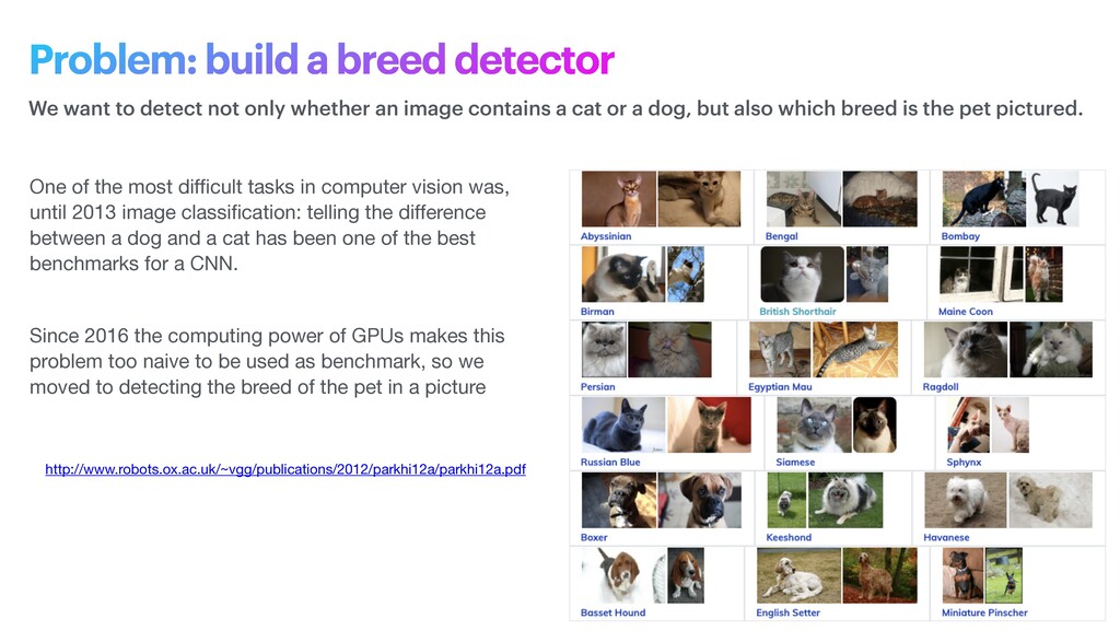
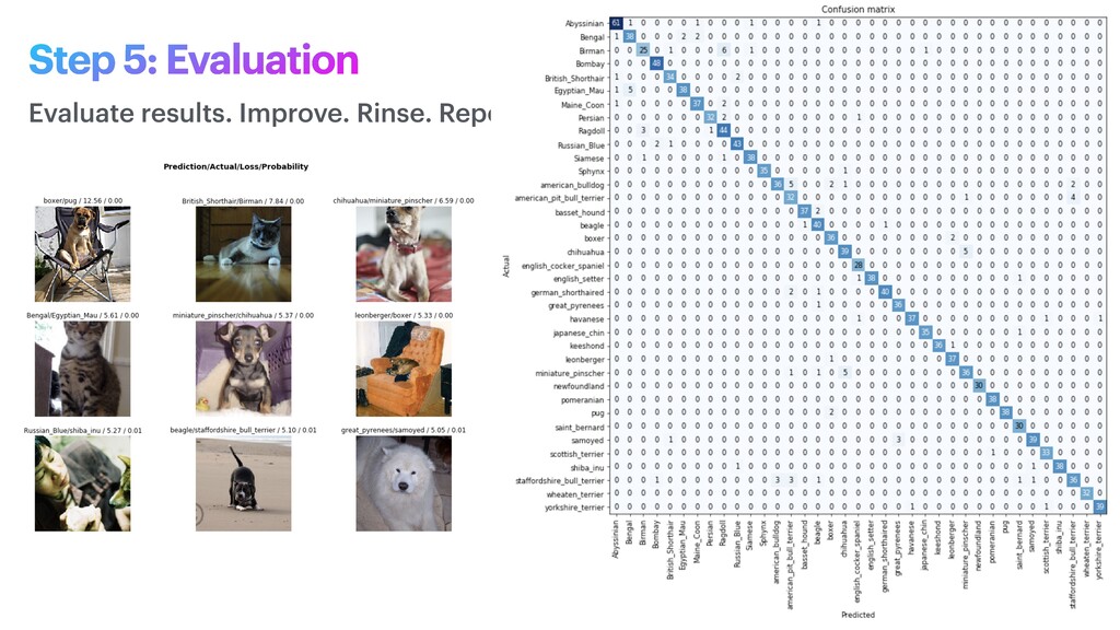
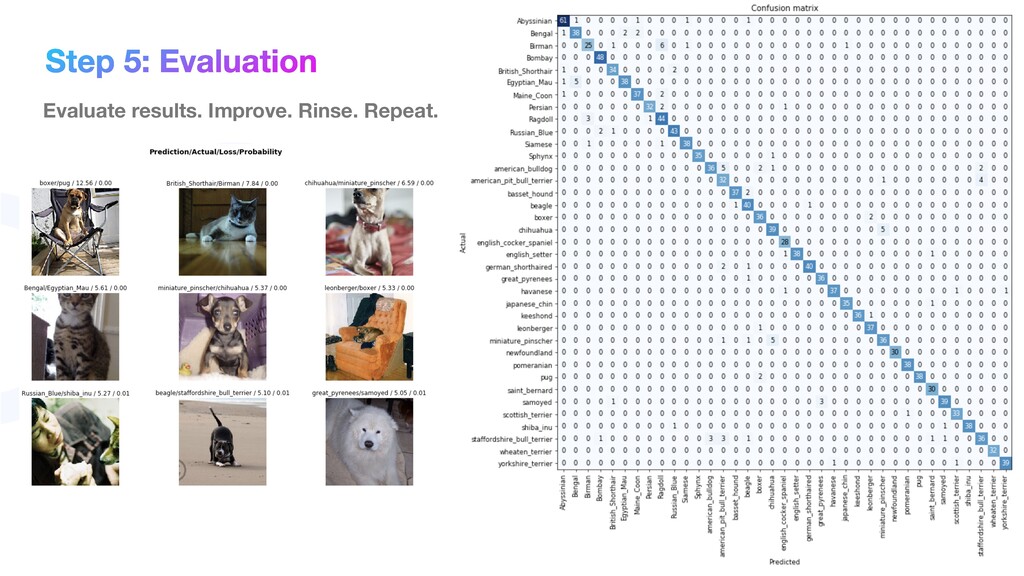
This phase is usually named data exploration and involves extracting some statistical
f
igures.
Step 1: Data Exploration
The first thing we do when we approach a problem is to take a
look at the data. We always need to understand very well what
the problem is and what the data looks like before we can figure
out how to solve it. Taking a look at the data means
understanding how the data directories are structured, what the
labels are and what some sample images look like.
Labels:
'Abyssinian', 'Bengal', 'Birman', 'Bombay', 'British_Shorthair', 'Egyptian_Mau', 'Maine_Coon',
'Persian', 'Ragdoll', 'Russian_Blue', 'Siamese', 'Sphynx', 'american_bulldog',
'american_pit_bull_terrier', 'basset_hound', 'beagle', 'boxer', 'chihuahua',
'english_cocker_spaniel', 'english_setter', 'german_shorthaired', 'great_pyrenees', 'havanese',
'japanese_chin', 'keeshond', 'leonberger', 'miniature_pinscher', 'newfoundland', 'pomeranian',
'pug', 'saint_bernard', 'samoyed', 'scottish_terrier', 'shiba_inu', 'staffordshire_bull_terrier',
'wheaten_terrier', 'yorkshire_terrier'

View Slide

In a real-life scenario data has not been prepared into a dataset for your convenience, but needs to be converted,
normalized and cleaned. Often datasets contain images that are blurred, too dark or simply wrong.

Finding the right amount of data needed for a classificator
● how different are the classes that you're trying to separate?

● how aggressively can you augment the training data?

● can you use pre-trained weights to initialise the lower layers of your net?

● do you plan to use batch normalisation?

● is dataset balanced or unbalanced?

A thumb rule would be starting with thousands of images, then extending your dataset as soon as more data is required
(i.e. error stops going down)
Remove outliers or unwanted data.
Step 2: Data Cleaning

View Slide

• All modern frameworks allow for dataset creation with augmentation techniques zooming,
f
lipping and rotating images. This makes your model robust to these transforms: the network
learns how to classify a pet also if the image is not perfectly captured or gets distorted for any
reason.

• More transforms your add, more images and training time you need.
If your model needs to be able to work with practical images, you need to “augment”
the batch set with rotations, skews and di
ff
erent sizes.
Step 3: Data Augmentation

View Slide

• Many CNN models come already pre-trained into Pytorch or Keras. Using a pre-trained model
and specializing the network on our dataset is often called transfer learning. Finding a good
metric is important to tell whether our model is over
f
itting a dataset (loss functions goes down,
error goes up).

• Some metrics are already built in, such as MSE, RMSE. FBeta, etc.
Choose your network architecture, a loss function and an error metric
Step 4: Training
learn = cnn_learner(data, models.resnet34, metrics=error_rate)
learn.fit_one_cycle(epocs)

View Slide

Evaluate results. Improve. Rinse. Repeat.
Step 5: Evaluation

View Slide

Section 4

View Slide

Solving Deep Learning
Module 7
A framework to solve real-live problems

View Slide

understanding your problem

View Slide

Slide Title
Structured data doesn’t need deep learning, but it could be “just” a machine learning or a big
data problem

View Slide

Slide Title
Unstructured data type, deep learning task, and business domain

View Slide

Slide Title
A Cambrian Explosion

View Slide

View Slide

a real-life scenario

View Slide

Real-Life Machine Learning Work
f
low

View Slide

1. Frame and understand your problem

2.Explore data with Analysis tools

3.Engineer features relevant to your use case

4.Partial train small models to build features

5.Explore existing pre-trained models to be adapted (i.e. using transfer learning)

6.Write speci
f
ic neural network code

7. Train, validate, evaluate ML model
Machine Learning starts before writing a single line of a neural network code
Implementing a ML model in real-life

View Slide

In this phase, the business problem is framed as a machine learning problem: what is observed
and what should be predicted (known as a label or target variable). Determining what to predict
and how performance and error metrics need to be optimized is a key step in ML.

For example, imagine a scenario where a manufacturing company wants to identify which products
will maximize pro
f
its. Reaching this business goal partially depends on determining the right number
of products to produce. In this scenario, you want to predict the future sales of the product, based on
past and current sales. Predicting future sales becomes the problem to solve, and using ML is one
approach that can be used to solve it.

ML problem framing

View Slide

• De
f
ine criteria for a successful outcome of the project

• Establish an observable and quanti
f
iable performance metric for the project, such as accuracy,
prediction latency, or minimizing inventory value

• Formulate the ML question in terms of inputs, desired outputs, and the performance metric to
be optimized

• Evaluate whether ML is a feasible and appropriate approach

• Create a data sourcing and data annotation objective, and a strategy to achieve it

• Start with a simple model that is easy to interpret, and which makes debugging more
manageable
ML problem framing

View Slide

Use cases
Module 8
Deep Learning application and use cases

in real life scenarios

View Slide

Use plain ResNet or VGG with transfer learning to find products within images coming from
catalogs or customer pictures.
Product auto-tagging and visual search
● Automatically tag products

● Cut down on workload to categorize products

● Show related products

● Find cheaper version of high end products

● Find complimentary products

● Find products usage on social media
https://www.kaggle.com/paramaggarwal/fashion-product-images-dataset

View Slide

Detect items not compliant with accepted sizes/shapes/colors.
Quality assurance
Real-time defect detection on a laser weld bead. a and c
show two side views of the weld bead where the blue
rectangles mark a defective section in the first and final
segments due to undercuts and the yellow ellipses mark a
region where some points have excessive porosity
CNNs approaches are capable of analysing MWIR
thermal images to extract parameters of laser
processes and quality indicators.

View Slide

Deep usage in security: detect accesses to restrict areas, detect people unhealthy behavior or
Self Driving cars
Uses a model ensenble to leverage
segmentation properties of CNNs.

CNNs to identify and segment, other ML
models to track cars and respond to
inputs

Lyft and Uber are experimenting self
driving cars for public transportation in
big cities such as Las Vegas.

View Slide

Use customer face as key to unlock credit card informations in a third party store
Payments using FaceID
Facebook Pay is experimenting payments
with face recognition.

AliPay just updated its proprietary
algorithm for face recognition to unlock
payments in store and personalized
advertising.

Libraries such as DLIB offer face
embeddings extraction and recognition
with an accuracy over 90%

View Slide

Multi-stage feature extraction and face rekognition. A CNN trained with triplet loss function
DLIB a face recognition library
Sometimes we have to train a network not to recognize a
given object, but to tell whether an image is or is not a given
person of interest.

A common technique is to define a particular loss function
named Triplet Loss.

DLIB network extracts landmarks from a face (named
measurements), then trains a network wit a known image
and two unknown different images.

This process makes the network able to understand
differences between pictures of any face.

View Slide

AI used for first time in job interviews in UK to find best applicants
CNNs used in recruiting
Unilever is among companies using AI technology
to analyse the language, tone and facial
expressions of candidates when they are asked a
set of identical job questions which they film on
their mobile phone or laptop.

The algorithms select the best applicants by
assessing their performances.

View Slide

China is the current biggest investor on Computer Vision applications, with focus on schools and
performance monitoring
CNNs in education
CNNs are used by China schools to monitor students attention
and posture, thus avoiding injuries or being too distracted
https://youtu.be/JMLsHI8aV0g?t=52

View Slide

Use CNNs to classify different sounds in an open environment
Environmental Sound Classification
Represent sound frequencies as images,
then classify different types of spectrum
to better classify sounds in an
environment

View Slide

Cancer Type Classification using CNN and Fast.AI
Neural Networks Applications in real life problems
https://towardsdatascience.com/the-mystery-of-the-origin-cancer-type-
classification-using-fast-ai-libray-212eaf8d3f4e

View Slide

Deep learning for patient‐specific quality assurance: Identifying errors in radiotherapy delivery by
radiomic analysis of gamma images with convolutional neural networks
Quality assurance in radiotherapy
CNNs can be used to detect operational errors when exposing patients to radiotherapy and provide a better
upfront correction of medical errors.

View Slide

Generate artificial images
GAN can be used to simulate face aging of
people in a natural and consistent way.

https://ieeexplore.ieee.org/document/8296650

View Slide

Used to train models in autonomous feedback-guided loops. It is used to implement variations of
autonomous driving agents.
Reinforcement Learning
Reinforcement Learning has a wide range of
applications from classification with a small dataset,
to playing video games, firewall/system parameters
tuning, personalizing reccomendations, automatic
bidding.

View Slide

Neosperience

Image Memorability

View Slide

What is a memorability score?
Image Memorability — A business perspective
Memorability is a measure of how much an image sticks into
the memory of an average customer respect to average
baseline images

A memorability score is a number representing memorability
of an image, compared to the average capability of a human
to remember an image which is 0.72

Images with a score higher than 0.72 have high memorability
and are suitable for campaigns

Images with a score lower than 0.72 underperform and should
be avoided because are not remembered

View Slide

A memorable image is a good image?
Image Memorability — A business perspective
High memorability score is a good starting point, but using it
to select an image could be too naive

More relevant than memorability itself is understanding which
feature makes an image memorable

Assigning a score to each pixel of the image regarding its
contribution to the resulting score

In this case memorability analysis outperforms humans
because it is able not only to tell the score

but also to understand what makes this score

View Slide

How to detect scores and heat maps?
Image Memorability — A technical perspective
Build an experiment to measure memorability (ground truth)

Deep Learning comes into help with CNNs

A CNN learns from experiment dataset how to estimate a memorability
score

From a given inference, finding layer activations (through back propagation)

Convolutions and back propagation are compute intensive tasks that
require GPUs even with inference

GPU inference is achieved through DeepLearning AMIs and on-premise
instances

We needed an architecture to support inference through GPU in production
in a scalable and cost effective way

View Slide

https://image.neosperience.com

View Slide

Neosperience

People Analytics

View Slide

Detect relevant insights about your customers in stores using cameras
Introducing Neosperience People Analytics
Neosperience Store Analytics is the SaaS solution to extract meaningful informations about people visiting
stores in an accurate and reliable way

● Uses both standard cameras and dedicated hardware with a cost effective profile

● Dedicated Hardware is projected to optimise costs, heat management and reliability

● Stream acquisition is achieved in cloud

● Allows for multiple people counting, detects unique visits

● Enables advanced insights extraction

View Slide

Mapping people presence within a given area of interest
Results: people heatmaps, trajectories, insight
Being able to recognise people and track their
movements in front of a camera leds to
interesting results not only related to people
counting

● Store managers can obtain a clear view of the
preferred areas inside a store

● And event the overall amount of people that
do not enter the store

● Store Analytics over delivered about store
understanding, delivering a different but more
meaningful metric

View Slide

Results
Results

View Slide

Results

View Slide

Alisea Visual Clean

View Slide

PROBLEM: Classify images of air duct/pipes as ‘dirty’ or ‘clean’
Alisea — Transfer learning example
Step 1: Exploratory analysis
Dataset composed of hundreds of images of different air pipes, taken with different cameras,
in different sizes.

Balanced dataset: 50% labelled ‘dirty’, 50% labelled ‘clean’.

RGB color channel.

Which images size to use? Which color channels?

View Slide

Step 2: Data Cleaning
Choose which images are appropriate for your training
dataset. Remove photos that would add ‘noise’. In our
case MANUALLY!

Considered image size:

● 128x128x3

● 256x256x3

● 320x320x3

● 480x480x3

Color channels:

● RGB, HSV
Not appropriate images for our dataset

View Slide

Step 3 & 4: Data augmentation and training
Data augmentation to increase image size.

Keras and other libraries allow you to import already trained CNNs, downloading both pretrained weights and
model architecture. Based on your need you can choose to keep the model as it is or:

● remove the fully connected (FC) layers at the end and add new layers that you need: Ex. final FC layer with
more output classes.

● Keep all the weights or train them all over again

Considered CNN architectures:

● ResNet34, ResNet50, ResNeXt50

Trained several models using different image sizes to notice if there was a difference in our results.

Best models in our case: ResNet50 and ResNeXt50

Best size: 256x256x3, bigger images need more computing power and longer training time

Best color channel: RGB

Final score: ~92% accuracy

View Slide

What does the model see?
Attention Heatmap
Feature Map of first Conv Layer

View Slide

Section 5

View Slide

PyTorch Lightning
Module 9
A framework to “reproducible” deep learning

View Slide

• Amazon SageMaker is a platform to run training and
inference from your laptop, directly in cloud.

• SageMaker training jobs allow setting up and tearing
down cloud infrastructure

• Can run training jobs locally on bare metal or
SageMaker containers
Amazon SageMaker
A Machine Learning platform

View Slide

PyTorch
• is pythonic (its n-dimensional tensor is similar to numpy) with a quite easy learning curve

• built-in support for data parallelism

• support for dynamic computational graphs

• Imperative programming model
A deep learning platform

View Slide

PyTorch on SageMaker
Running training on Amazon SageMaker
Initializes SageMaker session which holds context data
The bucket containig our input data
The IAM Role which SageMaker will impersonate to run the estimator

Remember you cannot use sagemaker.get_execution_role()

if you're not in a SageMaker notebook, an EC2 or a Lambda (i.e. running
from your local PC)
name of the runnable script containing __main__ function (entrypoint)
path of the folder containing training code. It could also contain a
requirements.txt
fi
le with all the dependencies that needs to be installed
before running
these hyperparameters are passed to the main script as arguments and can
be overridden when
fi
ne tuning the algorithm
Call
fi
t method on estimator, which trains our model, passing training and
testing datasets as environment variables. Data is copied from S3 before
initializing the container

View Slide

• A PyTorch implementation of MNIST
neural network is given.

• The network is built at forward pass.

• Each batch of data of each epoch
within train method
 
- loads data
 
- resets optimizer
 
- computes output
 
- computes loss
 
- optimizes weights
Amazon SageMaker

View Slide

Published in 2019, it is a framework to structure a PyTorch project,
gain support for less boilerplate and improved code reading.

The simple interface gives professional production
teams and newcomers access to the latest state of the art
techniques developed by the PyTorch and PyTorch Lightning
community.

• 96 contributors

• 8 research scientists

• rigorously tested
PyTorch Lightning
With Lightning, PyTorch gets both simpli
f
ied AND
on steroids
Principle 1 
Enable maximal
fl
exibility.

Principle 2 
Abstract away unnecessary boilerplate, but make it
accessible when needed.

Principle 3 
Systems should be self-contained (ie: optimizers,
computation code, etc).

Principle 4 
Deep learning code should be organized into 4 distinct
categories.

• Research code (the LightningModule).

• Engineering code (handled by the Trainer).

• Non-essential research code (in Callbacks).

• Data (PyTorch Dataloaders).

View Slide

Getting Started
Step 0: imports
Import PyTorch standard packages such as nn and Functional and
DataLoader
Import Transforms from torchvision (when needed)

Import pytorch_lightning core class

View Slide

Getting Started
Step 1: Lightning module
dataset preparation and loading
neural network de
fi
nition

loss computation

optimizers de
fi
nition
validation computation and stacking
Build a class extending pl.LightningModule and implement utility
methods which will be called by trainer during the training loop

View Slide

Getting Started
Step 2: Trainer
Lightning Trainer class controls
fl
ow execution, multi-GPU
parallelization and intermediary data saving to default_root_dir
Our de
fi
ned model class is istantiated passing all the required
hyperparams, then
fi
t method is called on trainer, passing params as
an argument

Training on multiple GPUs is easy as setting an argument

View Slide

Back to MNIST

View Slide

MNIST is the new Hello World
The MNIST database of handwritten digits has a training set
of 60,000 examples, and a test set of 10,000 examples. It is
a subset of a larger set available from NIST. The digits have
been size-normalized and centered in a
f
ixed-size image.

It is a good database for people who want to try learning
techniques and pattern recognition methods on real-world
data while spending minimal e
ff
orts on preprocessing and
formatting.
It’s a well known problem, that can be used as a reference

View Slide

SageMaker job script
Can be run from a Notebook or any Python environment
• Con
fi
gure SageMaker Session

• Setup an Estimator, con
fi
guring instance count, PyTorch container
version and instance type

• Pass training and testing datasets paths from S3. Data is copied
from S3 before initalizing the container and mapped to local folders

• After training containers get dismissed and instances destroyed

View Slide

Training class
Use PyTorch Lightning Trainer class
• Receives arguments from SageMaker (as arg variables)

• Instantiates a Trainer class

• Instantiates a classi
fi
er passing training parameters

• calls .
fi
t method on trainer, passing the model

• saves trained model to local model_dir which is mirrored to S3 by
SageMaker when container is dismissed

View Slide

MNISTClassi
f
ier

View Slide

PyTorch
 
https://pytorch.org/

PyTorch Lightning
 
https://github.com/PyTorchLightning/pytorch-lightning

PyTorch Lightning Bolts 
https://github.com/PyTorchLightning/pytorch-lightning-bolts
AWS re:Invent getting started video 
https://www.youtube.com/watch?v=6IhI7hPFpX8
Getting started with PL and Sagemaker
 
https://towardsdatascience.com/building-a-neural-network-on-amazon-sagemaker-with-pytorch-lightning-63730ec740ea
Useful resources

View Slide

Amazon SageMaker Platform
Module 10
Deep Learning applications, challenges, and tools

beyond Computer Vision

View Slide

• Amazon Customer Reviews Dataset

• https://s3.amazonaws.com/amazon-
reviews-pds/readme.html

• s3://amazon-reviews-pds/tsv/

• crawler with name “tsv”
 
• MSCK REPAIR TABLE tsv
Start exploring our dataset
Data collection

View Slide

Start exploring our dataset
Data collection

View Slide

Prepare data to be suitable for ML
Data preparation

View Slide

A work
f
low management tool for data analysis and preparation
SageMaker Data Wrangler

View Slide

O
ff
load SageMaker tasks to external workers
SageMaker Processing Platform

View Slide

• A single feature corresponds to a column in your dataset. A feature group is a prede
f
ined
schema for a collection of features - each feature in the feature group has a speci
f
ied data type
and name. A single record in a feature group corresponds to a row in your dataframe. A feature
store is a collection of feature groups.

• Record identi
f
ier name is the name of the feature de
f
ined in the feature group's feature
de
f
initions whose value uniquely identi
f
ies a Record de
f
ined in the feature group's feature
de
f
initions.

• Event time feature name is the name of the EventTime feature of a Record in FeatureGroup. An
EventTime is a timestamp that represents the point in time when a new event occurs that
corresponds to the creation or update of a Record in the FeatureGroup. All Records in the
FeatureGroup must have a corresponding EventTime.
SageMaker Feature Store

View Slide

• After the model has been trained, evaluate it to determine if its performance and accuracy will enable you
to achieve your business goals. You might want to generate multiple models using di
ff
erent methods and
evaluate the e
ff
ectiveness of each model. For example, you could apply di
ff
erent business rules for each
model, and then apply various measures to determine each model's suitability. You also might evaluate
whether your model needs to be more sensitive than speci
f
ic, or more speci
f
ic than sensitive. For
multiclass models, evaluate error rates for each class separately.

• You can evaluate your model using historical data (o
ff
line evaluation) or live data (online evaluation). In
o
ff
line evaluation, the trained model is evaluated with a portion of the dataset that has been set aside as
a holdout set. This holdout data is never used for model training or validation—it’s only used to evaluate
errors in the
f
inal model. The holdout data annotations need to have high accuracy for the evaluation to
make sense. Allocate additional resources to verify the accuracy of the holdout data.

• AWS services that are used for model training also have a role in this phase. Model validation can be
performed using Amazon SageMaker, AWS Deep Learning AMI, or Amazon EMR.

• Based on the evaluation results, you might
f
ine-tune the data, the algorithm, or both. When you
f
ine-tune
the data, you apply the concepts of data cleansing, preparation, and feature engineering.
How to know we arrived there?
Model Evaluation

View Slide

• Have a clear understanding of how you measure success

• Evaluate the model metrics against the business expectations for the project

• Plan and execute Production Deployment (Model Deployment and Model Inference)

Apply these best practices:

• Monitor model performance in production and compare to business expectations

• Monitor di
ff
erences between model performance during training and in production

• When changes in model performance are detected, retrain the model. For example, sales expectations
and subsequent predictions may change due to new competition

• Use batch transform as an alternative to hosting services if you want to get inferences on entire
datasets

• Take advantage of production variants to test variations of a new model with A/B testing
How to know we arrived there?
Model Evaluation

View Slide

AWS ML Stack

View Slide

The AWS machine learning stack
Broadest and most complete set of Machine Learning capabilities

View Slide

Thesis Proposals

View Slide

Books and bibliography

View Slide

Resources
What to expect from AI
Immortality or Extinction 
https://waitbutwhy.com/2015/01/arti
fi
cial-intelligence-revolution-1.html
The Hyperion Cycle
Dan Simmons

View Slide

View Slide

thank you.

View Slide

2021 Computer Vision with CNN

2021 Computer Vision with CNN

Aletheia

More Decks by Aletheia

Other Decks in Technology

Featured

Transcript