Computação científica com Python - Grupy-SP, agosto de 2015

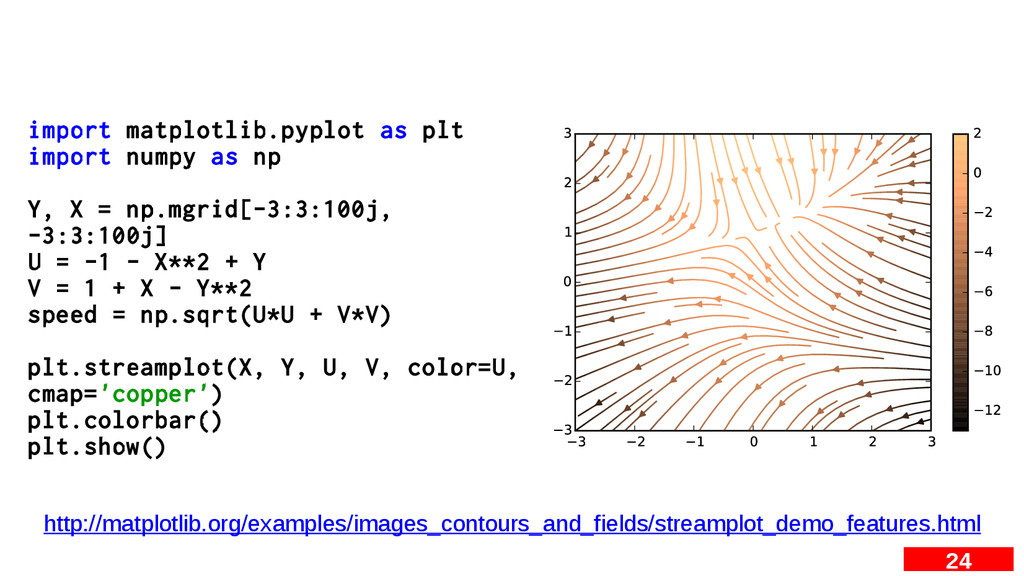
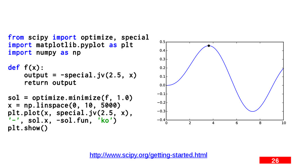
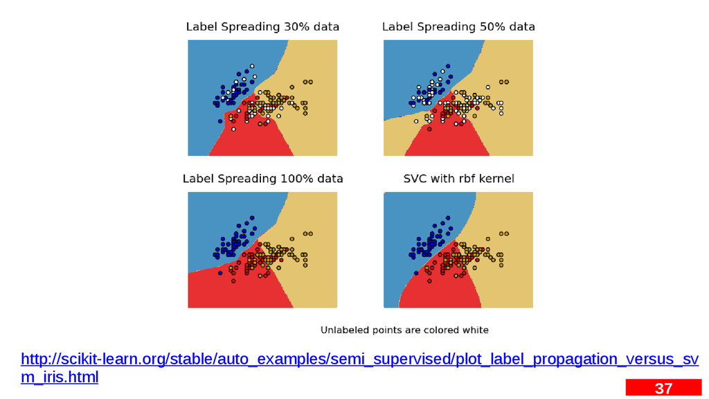
Nesta palestra foram abordadas noções preliminares de Python voltado à computação científica. Foram apresentados pacotes de extensão, como numpy, scipy, matplotlib, scikit-learn, scikit-image, entre outros. O objetivo é disseminar o uso de software livre em aplicações científicas por meio de universidades, laboratórios e instituições de ensino.

Transcript

1. Computação científica com Python Alexandre de Siqueira
2. 2 Por que Python?
3. 3 Por que não uma linguagem compilada?
4. 4 C / C++: menos produtivo
5. 5 Fortran: • menos produtivo • restrito
6. 6 Por que não outra linguagem interpretada?
7. 7 Matlab / Octave: • restrito • lento • caro
8. 8 R: curva de aprendizado maior
9. 9 Julia: poucos pacotes
10. 10 “Every tool has its place”.
11. 11 Python: • adoção confusa (2 ou 3?) • lento
12. 12 Vamos falar de Python :)
13. 13 Qual a melhor distribuição?
14. 14 sudo VS
15. 15 $ sudo apt-get install idle- python3.4 ipython3-qtconsole python3-numpy python3-scipy python3-matplotlib mayavi2 python3-pandas python3- skimage python3-simpy...
16. 16 $ bash Anaconda3-2.3.0-Linux- x86_64.sh
17. 17 $ conda install <pacote>
18. 18 E o ambiente?
19. 19 ? ? idle? ?
20. 20 $ conda install spyder
21. 21 https://github.com/spyder-ide/spyder
22. 22 E o que posso fazer com isso?
23. 23 • o básico
24. 24 import matplotlib.pyplot as plt import numpy as np Y, X = np.mgrid[-3:3:100j, -3:3:100j] U = -1 - X**2 + Y V = 1 + X - Y**2 speed = np.sqrt(U*U + V*V) plt.streamplot(X, Y, U, V, color=U, cmap='copper') plt.colorbar() plt.show() http://matplotlib.org/examples/images_contours_and_fields/streamplot_demo_features.html
25. 25 from mpl_toolkits.mplot3d import axes3d import matplotlib.pyplot as plt import numpy as np fig = plt.figure() ax = fig.add_subplot(111, projection='3d') X, Y, Z = axes3d.get_test_data(0.05) ax.plot_wireframe(X, Y, Z, rstride=10, cstride=10) plt.show() http://matplotlib.org/examples/mplot3d/wire3d_demo.html
26. 26 from scipy import optimize, special import matplotlib.pyplot as plt import numpy as np def f(x): output = -special.jv(2.5, x) return output sol = optimize.minimize(f, 1.0) x = np.linspace(0, 10, 5000) plt.plot(x, special.jv(2.5, x), '-', sol.x, -sol.fun, 'ko') plt.show() http://www.scipy.org/getting-started.html
27. 27 • matemática simbólica
28. 28 In [30]: from sympy import * In [31]: f, g = symbols('f g', cls=Function) In [32]: f(x) Out[32]: f(x) In [33]: f(x).diff(x) Out[33]: Derivative(f(x), x) In [34]: diffeq = Eq(f(x).diff(x, x) - 2*f(x).diff(x) + f(x), sin(x)) In [35]: diffeq Out[35]: f(x) - 2*Derivative(f(x), x) + Derivative(f(x), x, x) == sin(x) In [36]: dsolve(diffeq, f(x)) Out[36]: f(x) == (C1 + C2*x)*exp(x) + cos(x)/2 http://docs.sympy.org/latest/tutorial/solvers.html#solving-differential-equations
29. 29 • estatística seaborn
30. 30 from scipy.stats import kendalltau import numpy as np import seaborn as sns sns.set(style="ticks") rs = np.random.RandomState(11) x = rs.gamma(2, size=1000) y = -.5 * x + rs.normal(size=1000) sns.jointplot(x, y, kind="hex", stat_func=kendalltau, color="#4CB391") http://stanford.edu/~mwaskom/software/seaborn/examples/hexbin_marginals.html
31. 31 import pandas as pd import random as rd import seaborn as sns df = pd.DataFrame() df['x'] = rd.sample(range(1, 100), 75) df['y'] = rd.sample(range(1, 100), 75) sns.lmplot('x', 'y', data=df, fit_reg=False) sns.kdeplot(df.y, df.x) http://chrisalbon.com/python/pandas_with_seaborn.html
32. 32 • processamento de imagens
33. 33 from skimage import data from skimage.filters import threshold_otsu, threshold_adaptive import matplotlib.pyplot as plt image = data.page() global_thresh = threshold_otsu(image) binary_global = image > global_thresh block_size = 40 binary_adaptive = threshold_adaptive(image, block_size, offset=10) fig, axes = plt.subplots(nrows=3, figsize=(7, 8)) ax0, ax1, ax2 = axes plt.gray() ax0.imshow(image) ax1.imshow(binary_global) ax2.imshow(binary_adaptive) for ax in axes: ax.axis('off') plt.show() http://scikit-image.org/docs/dev/auto_examples/plot_threshold_adaptive.html
34. 34 from skimage import data from skimage.filters.rank import entropy from skimage.morphology import disk from skimage.util import img_as_ubyte import matplotlib.pyplot as plt image = img_as_ubyte(data.camera()) fig, (ax0, ax1) = plt.subplots(nrows=2, figsize=(4, 8)) img0 = ax0.imshow(image, cmap=plt.cm.gray) ax0.set_title('Image') ax0.axis('off') img1 = ax1.imshow(entropy(image, disk(5)), cmap=plt.cm.jet) ax1.set_title('Entropy') ax1.axis('off') plt.show() http://scikit-image.org/docs/dev/auto_examples/plot_entropy.html
35. 35 • aprendizagem de máquina
36. 36 http://scikit-learn.org/stable/auto_examples/covariance/plot_outlier_detection.html
37. 37 http://scikit-learn.org/stable/auto_examples/semi_supervised/plot_label_propagation_versus_sv m_iris.html
38. 38 e muitos outros! https://pypi.python.org/pypi?:action=browse&c=385
39. 39 Obrigado! • contato: www.programandociencia.com/sobre