Sample Size Re-Estimation

The sample size re-estimation module for the "Adaptive and Bayesian Methods for Clinical Trial Design Short Course" by Dr. Alex Kaizer.

Transcript

1. Adaptive and Bayesian Methods for Clinical Trial Design Short Course Dr. Alex Kaizer Sample Size Re-Estimation
2. Some Background and Logistics Some of the practical considerations 2
3. Overview Paper: 3
4. Terminology 4 Separate module!
5. Background Sample size re-estimation, when one power calculation isn’t enough! 5
6. Why Adapt the Sample Size? Hypothetical Scenario: • You design and power a study on a research topic with limited prior information (i.e., there is uncertainty in your sample size calculation assumptions) • As the study is being conducted, the observed treatment effect is smaller than expected, but still clinically meaningful • If we maintain the planned sample size, we may be underpowered to detect this difference 6 Image Source: Everyday Health
7. Purpose • Sample size re-estimation allows a study to modify the planned sample size based on accumulating data to account for uncertainty of power calculations conducted during the initial design • Re-estimation can increase likelihood of a “successful” trial, but may also lead to a substantial increase in the needed sample size • Many methods exist with different considerations for any given study 7
8. Categories of Re-Estimation Approaches Two categories of re-estimation procedures exist with regards to knowledge of study arm allocation of randomized participants: • Blinded • Study arm allocation not known • Often used to estimate nuisance parameters (e.g., variance of continuous outcome, overall event rate, etc.) to revise pre-study assumed value • Little concerns with control of type I error rate • Unblinded • Study arm allocation is known • Often used to estimate the effect size and potentially nuisance parameters to use in revising pre-study values • Concerns with control of the type I error rate (similar to efficacy interim analyses) 8
9. Blinded Re-Estimation Methods Putting the “new” in nuisance (parameter) 9
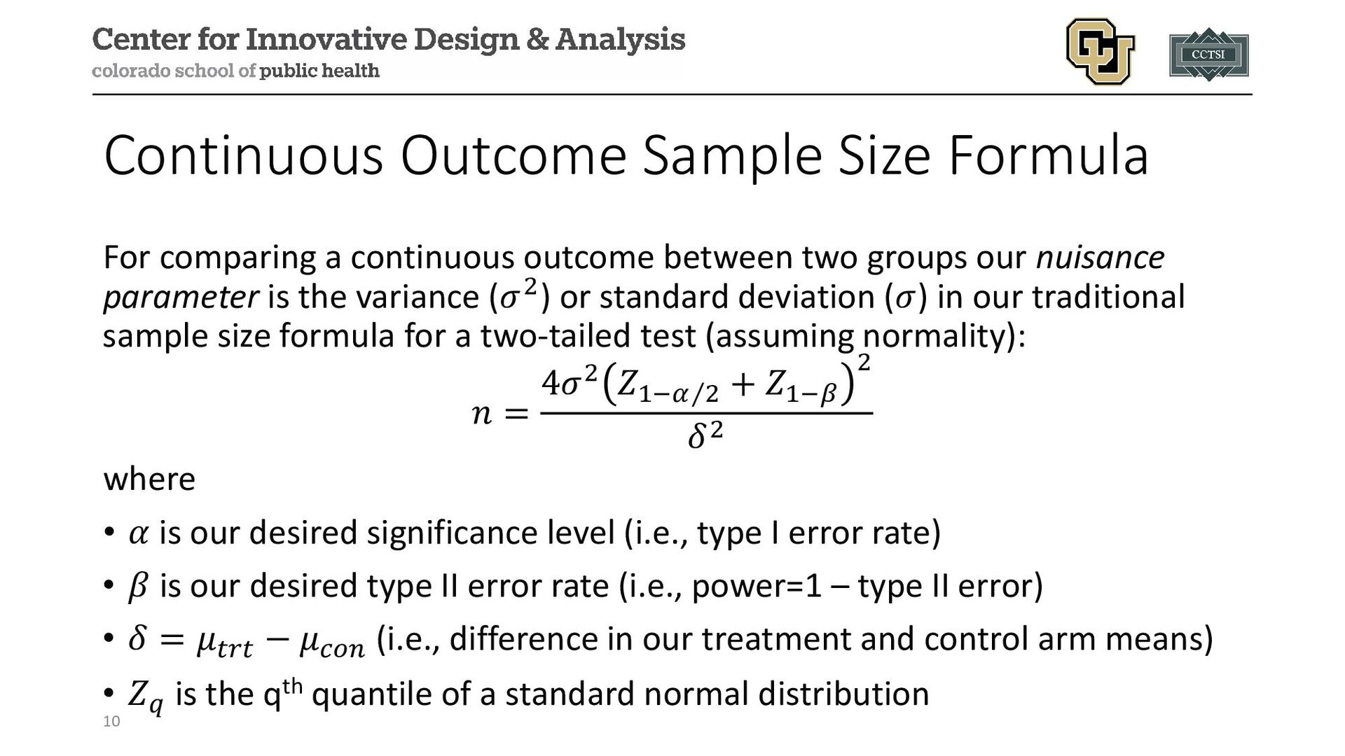
10. Continuous Outcome Sample Size Formula For comparing a continuous outcome between two groups our nuisance parameter is the variance (𝜎𝜎2) or standard deviation (𝜎𝜎) in our traditional sample size formula for a two-tailed test (assuming normality): 𝑛𝑛 = 4𝜎𝜎2 𝑍𝑍1− ⁄ 𝛼𝛼 2 + 𝑍𝑍1−𝛽𝛽 2 𝛿𝛿2 where • 𝛼𝛼 is our desired significance level (i.e., type I error rate) • 𝛽𝛽 is our desired type II error rate (i.e., power=1 – type II error) • 𝛿𝛿 = 𝜇𝜇𝑡𝑡𝑡𝑡𝑡𝑡 − 𝜇𝜇𝑐𝑐𝑐𝑐𝑐𝑐 (i.e., difference in our treatment and control arm means) • 𝑍𝑍𝑞𝑞 is the qth quantile of a standard normal distribution 10
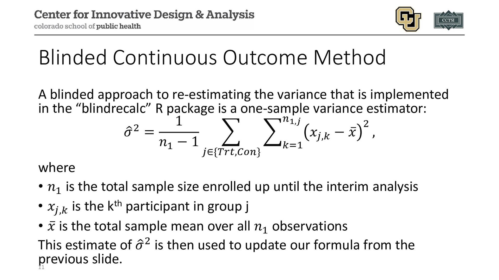
11. Blinded Continuous Outcome Method A blinded approach to re-estimating the variance that is implemented in the “blindrecalc” R package is a one-sample variance estimator: � 𝜎𝜎2 = 1 𝑛𝑛1 − 1 � 𝑗𝑗∈{𝑇𝑇𝑇𝑇𝑇𝑇,𝐶𝐶𝐶𝐶𝐶𝐶} � 𝑘𝑘=1 𝑛𝑛1,𝑗𝑗 𝑥𝑥𝑗𝑗,𝑘𝑘 − ̅ 𝑥𝑥 2 , where • 𝑛𝑛1 is the total sample size enrolled up until the interim analysis • 𝑥𝑥𝑗𝑗,𝑘𝑘 is the kth participant in group j • ̅ 𝑥𝑥 is the total sample mean over all 𝑛𝑛1 observations This estimate of � 𝜎𝜎2 is then used to update our formula from the previous slide. 11
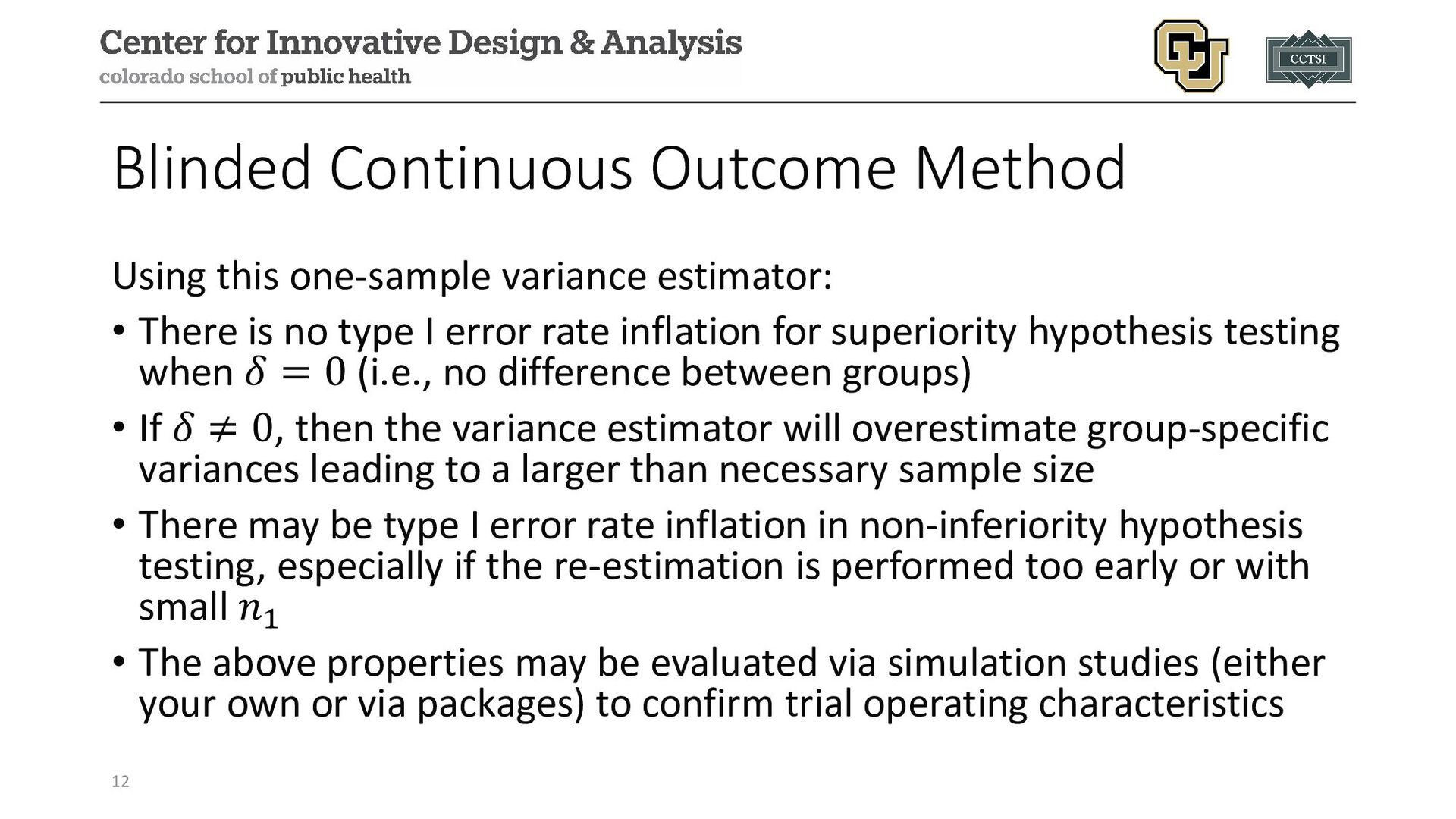
12. Blinded Continuous Outcome Method Using this one-sample variance estimator: • There is no type I error rate inflation for superiority hypothesis testing when 𝛿𝛿 = 0 (i.e., no difference between groups) • If 𝛿𝛿 ≠ 0, then the variance estimator will overestimate group-specific variances leading to a larger than necessary sample size • There may be type I error rate inflation in non-inferiority hypothesis testing, especially if the re-estimation is performed too early or with small 𝑛𝑛1 • The above properties may be evaluated via simulation studies (either your own or via packages) to confirm trial operating characteristics 12
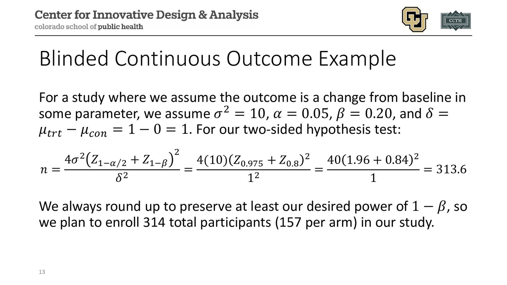
13. Blinded Continuous Outcome Example For a study where we assume the outcome is a change from baseline in some parameter, we assume 𝜎𝜎2 = 10, 𝛼𝛼 = 0.05, 𝛽𝛽 = 0.20, and 𝛿𝛿 = 𝜇𝜇𝑡𝑡𝑡𝑡𝑡𝑡 − 𝜇𝜇𝑐𝑐𝑐𝑐𝑐𝑐 = 1 − 0 = 1. For our two-sided hypothesis test: 𝑛𝑛 = 4𝜎𝜎2 𝑍𝑍1− ⁄ 𝛼𝛼 2 + 𝑍𝑍1−𝛽𝛽 2 𝛿𝛿2 = 4(10) 𝑍𝑍0.975 + 𝑍𝑍0.8 2 12 = 40 1.96 + 0.84 2 1 = 313.6 We always round up to preserve at least our desired power of 1 − 𝛽𝛽, so we plan to enroll 314 total participants (157 per arm) in our study. 13
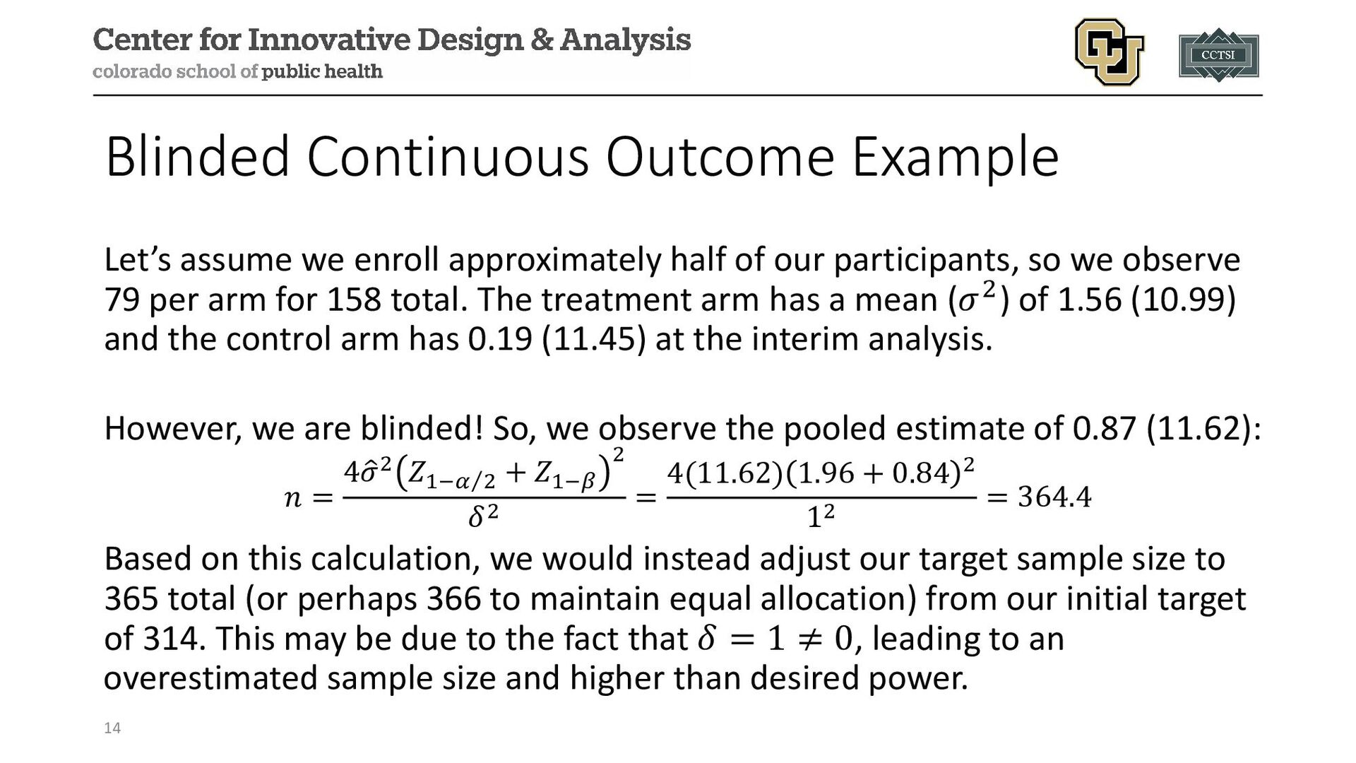
14. Blinded Continuous Outcome Example Let’s assume we enroll approximately half of our participants, so we observe 79 per arm for 158 total. The treatment arm has a mean (𝜎𝜎2) of 1.56 (10.99) and the control arm has 0.19 (11.45) at the interim analysis. However, we are blinded! So, we observe the pooled estimate of 0.87 (11.62): 𝑛𝑛 = 4 � 𝜎𝜎2 𝑍𝑍1− ⁄ 𝛼𝛼 2 + 𝑍𝑍1−𝛽𝛽 2 𝛿𝛿2 = 4(11.62) 1.96 + 0.84 2 12 = 364.4 Based on this calculation, we would instead adjust our target sample size to 365 total (or perhaps 366 to maintain equal allocation) from our initial target of 314. This may be due to the fact that 𝛿𝛿 = 1 ≠ 0, leading to an overestimated sample size and higher than desired power. 14
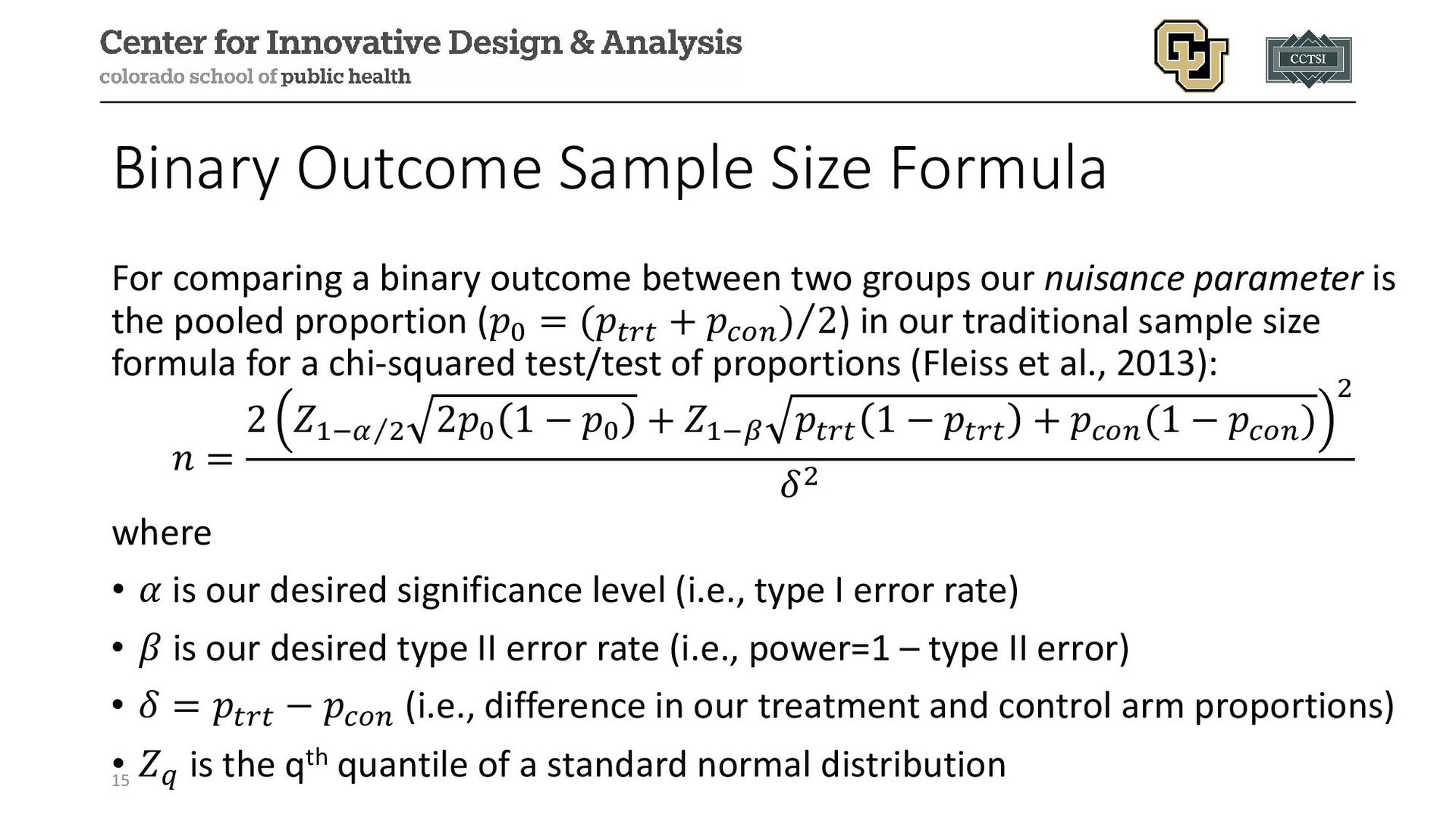
15. Binary Outcome Sample Size Formula For comparing a binary outcome between two groups our nuisance parameter is the pooled proportion (𝑝𝑝0 = ⁄ (𝑝𝑝𝑡𝑡𝑡𝑡𝑡𝑡 + 𝑝𝑝𝑐𝑐𝑐𝑐𝑐𝑐 ) 2) in our traditional sample size formula for a chi-squared test/test of proportions (Fleiss et al., 2013): 𝑛𝑛 = 2 𝑍𝑍1− ⁄ 𝛼𝛼 2 2𝑝𝑝0 1 − 𝑝𝑝0 + 𝑍𝑍1−𝛽𝛽 𝑝𝑝𝑡𝑡𝑡𝑡𝑡𝑡 1 − 𝑝𝑝𝑡𝑡𝑡𝑡𝑡𝑡 + 𝑝𝑝𝑐𝑐𝑐𝑐𝑐𝑐 (1 − 𝑝𝑝𝑐𝑐𝑐𝑐𝑐𝑐 ) 2 𝛿𝛿2 where • 𝛼𝛼 is our desired significance level (i.e., type I error rate) • 𝛽𝛽 is our desired type II error rate (i.e., power=1 – type II error) • 𝛿𝛿 = 𝑝𝑝𝑡𝑡𝑡𝑡𝑡𝑡 − 𝑝𝑝𝑐𝑐𝑐𝑐𝑐𝑐 (i.e., difference in our treatment and control arm proportions) • 𝑍𝑍𝑞𝑞 is the qth quantile of a standard normal distribution 15
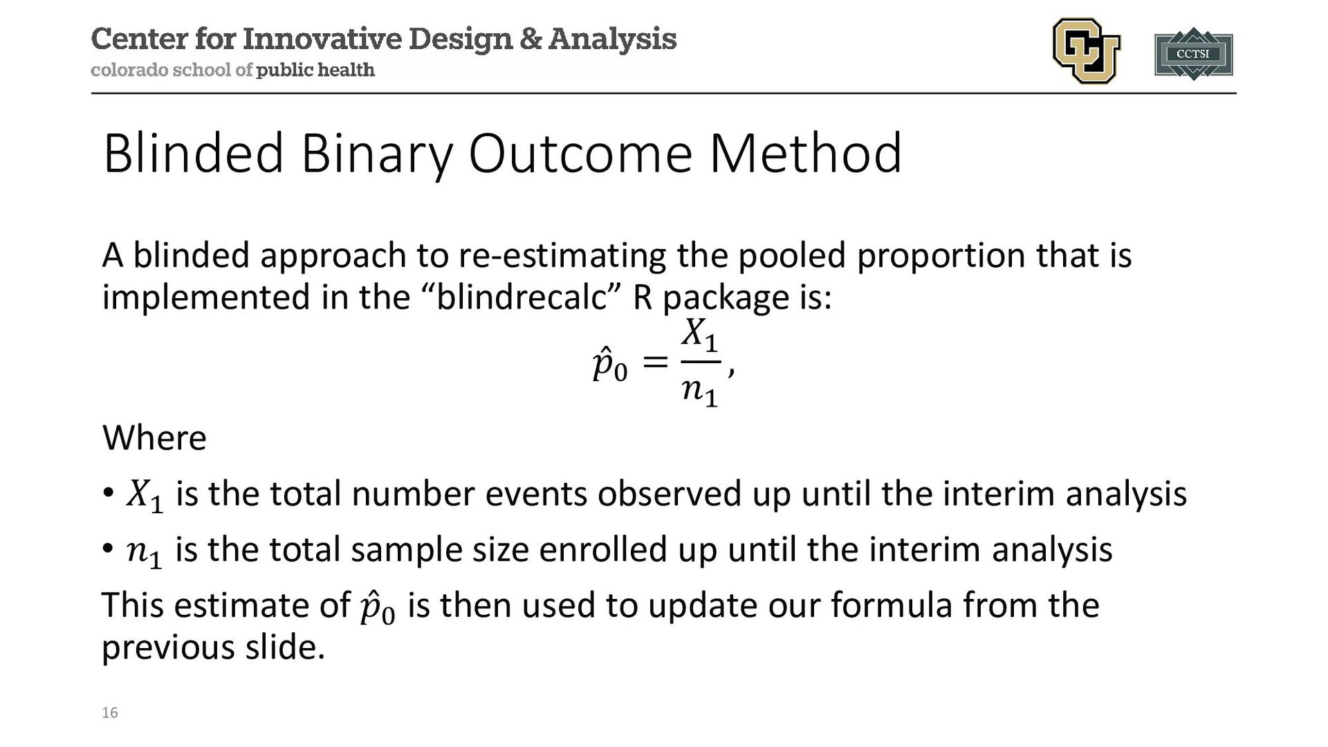
16. Blinded Binary Outcome Method A blinded approach to re-estimating the pooled proportion that is implemented in the “blindrecalc” R package is: ̂ 𝑝𝑝0 = 𝑋𝑋1 𝑛𝑛1 , Where • 𝑋𝑋1 is the total number events observed up until the interim analysis • 𝑛𝑛1 is the total sample size enrolled up until the interim analysis This estimate of ̂ 𝑝𝑝0 is then used to update our formula from the previous slide. 16
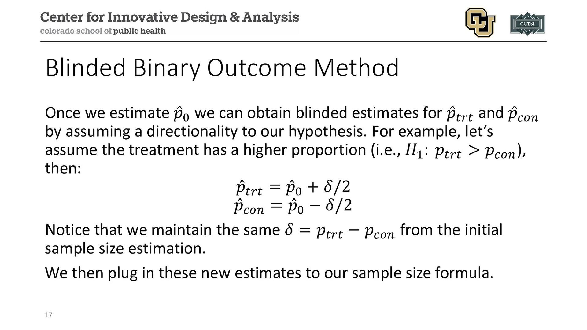
17. Blinded Binary Outcome Method Once we estimate ̂ 𝑝𝑝0 we can obtain blinded estimates for ̂ 𝑝𝑝𝑡𝑡𝑡𝑡𝑡𝑡 and ̂ 𝑝𝑝𝑐𝑐𝑐𝑐𝑐𝑐 by assuming a directionality to our hypothesis. For example, let’s assume the treatment has a higher proportion (i.e., 𝐻𝐻1 : 𝑝𝑝𝑡𝑡𝑡𝑡𝑡𝑡 > 𝑝𝑝𝑐𝑐𝑐𝑐𝑐𝑐), then: ̂ 𝑝𝑝𝑡𝑡𝑡𝑡𝑡𝑡 = ̂ 𝑝𝑝0 + 𝛿𝛿/2 ̂ 𝑝𝑝𝑐𝑐𝑐𝑐𝑐𝑐 = ̂ 𝑝𝑝0 − 𝛿𝛿/2 Notice that we maintain the same 𝛿𝛿 = 𝑝𝑝𝑡𝑡𝑡𝑡𝑡𝑡 − 𝑝𝑝𝑐𝑐𝑐𝑐𝑐𝑐 from the initial sample size estimation. We then plug in these new estimates to our sample size formula. 17
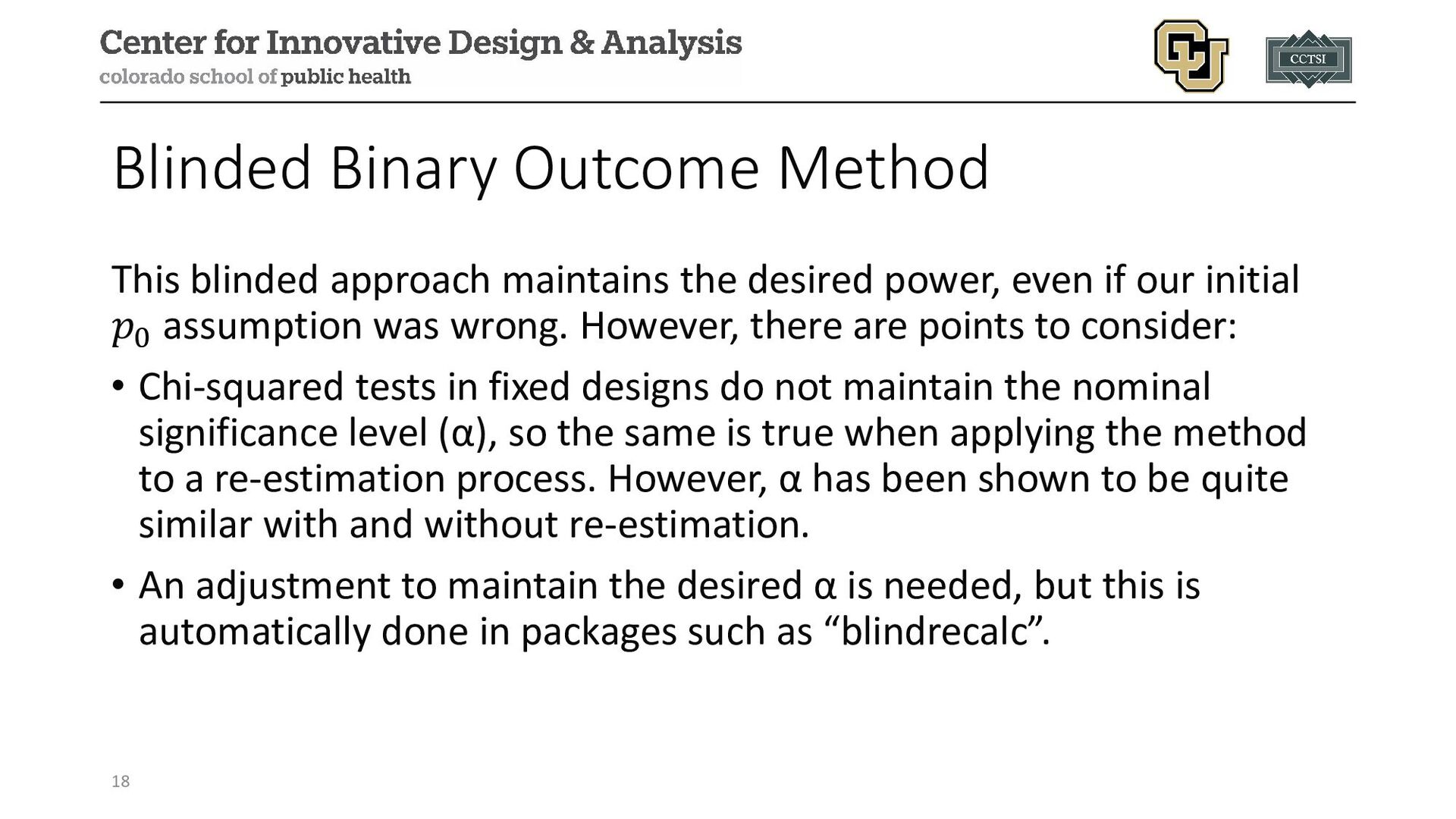
18. Blinded Binary Outcome Method This blinded approach maintains the desired power, even if our initial 𝑝𝑝0 assumption was wrong. However, there are points to consider: • Chi-squared tests in fixed designs do not maintain the nominal significance level (α), so the same is true when applying the method to a re-estimation process. However, α has been shown to be quite similar with and without re-estimation. • An adjustment to maintain the desired α is needed, but this is automatically done in packages such as “blindrecalc”. 18
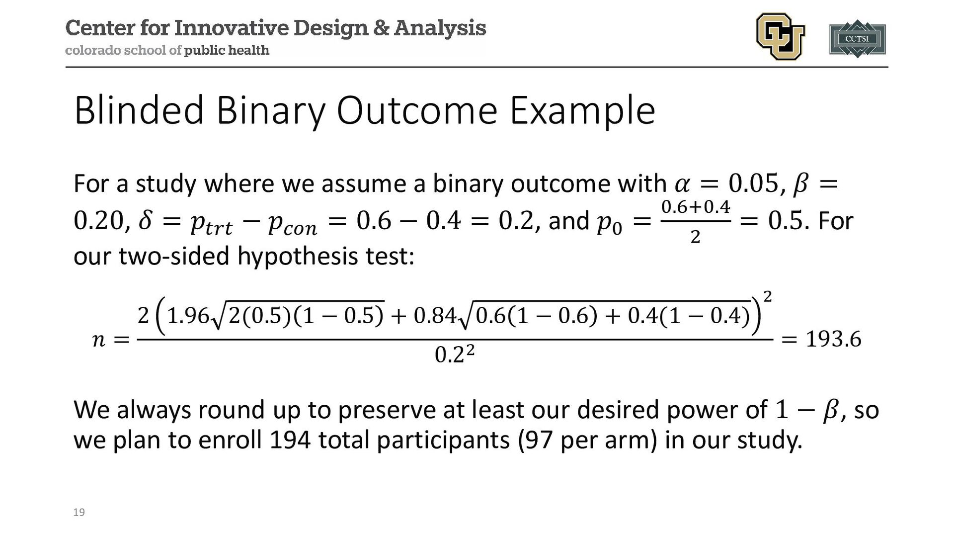
19. Blinded Binary Outcome Example For a study where we assume a binary outcome with 𝛼𝛼 = 0.05, 𝛽𝛽 = 0.20, 𝛿𝛿 = 𝑝𝑝𝑡𝑡𝑡𝑡𝑡𝑡 − 𝑝𝑝𝑐𝑐𝑐𝑐𝑐𝑐 = 0.6 − 0.4 = 0.2, and 𝑝𝑝0 = 0.6+0.4 2 = 0.5. For our two-sided hypothesis test: 𝑛𝑛 = 2 1.96 2(0.5) 1 − 0.5 + 0.84 0.6 1 − 0.6 + 0.4(1 − 0.4) 2 0.22 = 193.6 We always round up to preserve at least our desired power of 1 − 𝛽𝛽, so we plan to enroll 194 total participants (97 per arm) in our study. 19
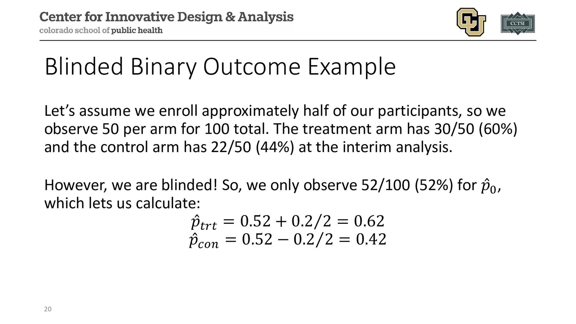
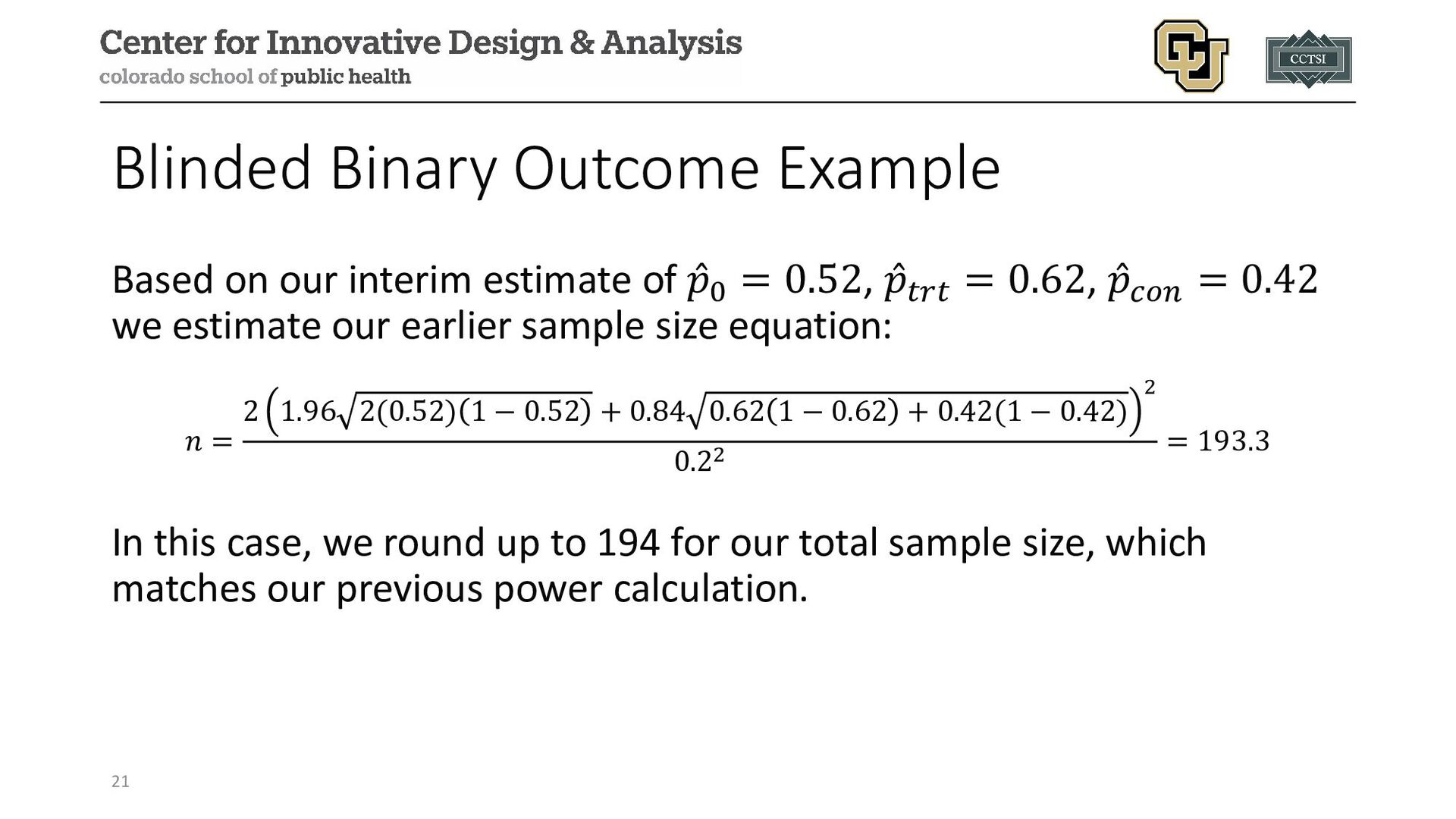
20. Blinded Binary Outcome Example Let’s assume we enroll approximately half of our participants, so we observe 50 per arm for 100 total. The treatment arm has 30/50 (60%) and the control arm has 22/50 (44%) at the interim analysis. However, we are blinded! So, we only observe 52/100 (52%) for ̂ 𝑝𝑝0, which lets us calculate: ̂ 𝑝𝑝𝑡𝑡𝑡𝑡𝑡𝑡 = 0.52 + ⁄ 0.2 2 = 0.62 ̂ 𝑝𝑝𝑐𝑐𝑐𝑐𝑐𝑐 = 0.52 − ⁄ 0.2 2 = 0.42 20
21. Blinded Binary Outcome Example Based on our interim estimate of ̂ 𝑝𝑝0 = 0.52, ̂ 𝑝𝑝𝑡𝑡𝑡𝑡𝑡𝑡 = 0.62, ̂ 𝑝𝑝𝑐𝑐𝑐𝑐𝑐𝑐 = 0.42 we estimate our earlier sample size equation: 𝑛𝑛 = 2 1.96 2(0.52) 1 − 0.52 + 0.84 0.62 1 − 0.62 + 0.42(1 − 0.42) 2 0.22 = 193.3 In this case, we round up to 194 for our total sample size, which matches our previous power calculation. 21
22. Blinded Re-estimation for Binary Outcome with Blocked Randomization Method • It is also possible to maintain blinding while estimating group-specific treatment effects based on a clever application of block randomization. • We will explore the proposed method by Shih and Peng-Liang (1997) in the following slides. 22
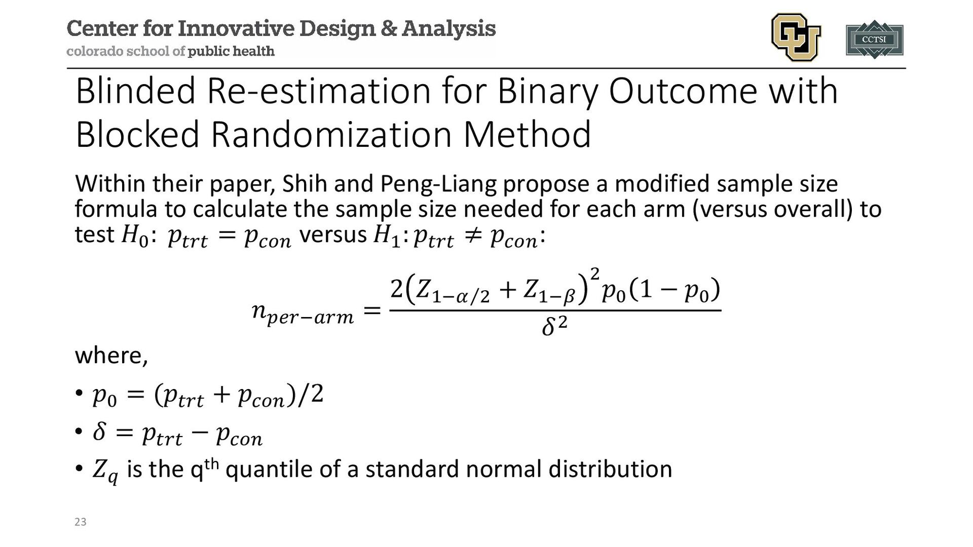
23. Blinded Re-estimation for Binary Outcome with Blocked Randomization Method Within their paper, Shih and Peng-Liang propose a modified sample size formula to calculate the sample size needed for each arm (versus overall) to test 𝐻𝐻0 : 𝑝𝑝𝑡𝑡𝑡𝑡𝑡𝑡 = 𝑝𝑝𝑐𝑐𝑐𝑐𝑐𝑐 versus 𝐻𝐻1 : 𝑝𝑝𝑡𝑡𝑡𝑡𝑡𝑡 ≠ 𝑝𝑝𝑐𝑐𝑐𝑐𝑐𝑐: 𝑛𝑛𝑝𝑝𝑝𝑝𝑝𝑝−𝑎𝑎𝑎𝑎𝑎𝑎 = 2 𝑍𝑍 ⁄ 1−𝛼𝛼 2 + 𝑍𝑍1−𝛽𝛽 2 𝑝𝑝0 1 − 𝑝𝑝0 𝛿𝛿2 where, • 𝑝𝑝0 = (𝑝𝑝𝑡𝑡𝑡𝑡𝑡𝑡 + 𝑝𝑝𝑐𝑐𝑐𝑐𝑐𝑐 )/2 • 𝛿𝛿 = 𝑝𝑝𝑡𝑡𝑡𝑡𝑡𝑡 − 𝑝𝑝𝑐𝑐𝑐𝑐𝑐𝑐 • 𝑍𝑍𝑞𝑞 is the qth quantile of a standard normal distribution 23
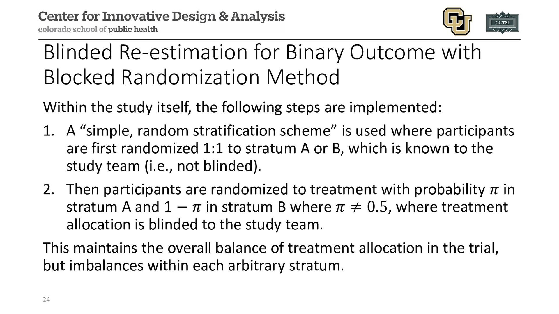
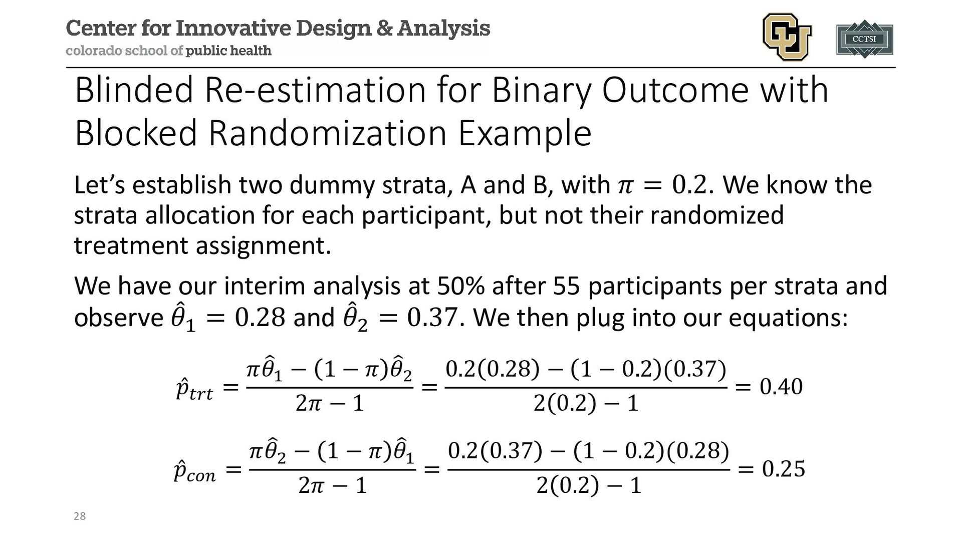
24. Blinded Re-estimation for Binary Outcome with Blocked Randomization Method Within the study itself, the following steps are implemented: 1. A “simple, random stratification scheme” is used where participants are first randomized 1:1 to stratum A or B, which is known to the study team (i.e., not blinded). 2. Then participants are randomized to treatment with probability 𝜋𝜋 in stratum A and 1 − 𝜋𝜋 in stratum B where 𝜋𝜋 ≠ 0.5, where treatment allocation is blinded to the study team. This maintains the overall balance of treatment allocation in the trial, but imbalances within each arbitrary stratum. 24
25. Blinded Re-estimation for Binary Outcome with Blocked Randomization Method At the interim analysis, we estimate the stratum as: • Stratum A: 𝜃𝜃1 = 𝑃𝑃 𝑦𝑦𝑗𝑗 = 1 𝑝𝑝𝑝𝑝𝑝𝑝𝑝𝑝𝑝𝑝𝑝𝑝𝑝𝑝𝑝𝑝𝑝𝑝𝑝𝑝𝑝𝑝 𝑗𝑗 ∈ 𝑠𝑠𝑠𝑠𝑠𝑠𝑠𝑠𝑠𝑠𝑠𝑠𝑠𝑠 𝐴𝐴 = 𝜋𝜋𝑝𝑝𝑡𝑡𝑡𝑡𝑡𝑡 + 1 − 𝜋𝜋 𝑝𝑝𝑐𝑐𝑐𝑐𝑐𝑐 • Stratum B: 𝜃𝜃2 = 𝑃𝑃 𝑦𝑦𝑗𝑗 = 1 𝑝𝑝𝑝𝑝𝑝𝑝𝑝𝑝𝑝𝑝𝑝𝑝𝑝𝑝𝑝𝑝𝑝𝑝𝑝𝑝𝑝𝑝 𝑗𝑗 ∈ 𝑠𝑠𝑠𝑠𝑠𝑠𝑠𝑠𝑠𝑠𝑠𝑠𝑠𝑠 𝐵𝐵 = (1 − 𝜋𝜋)𝑝𝑝𝑡𝑡𝑡𝑡𝑡𝑡 + 𝜋𝜋𝑝𝑝𝑐𝑐𝑐𝑐𝑐𝑐 The observed rates ̂ 𝜃𝜃𝑘𝑘 are unbiased estimators for 𝜃𝜃𝑘𝑘. These equations can be solved for: ̂ 𝑝𝑝𝑡𝑡𝑡𝑡𝑡𝑡 = 𝜋𝜋 � 𝜃𝜃1 − 1 − 𝜋𝜋 � 𝜃𝜃2 2𝜋𝜋 − 1 ̂ 𝑝𝑝𝑐𝑐𝑐𝑐𝑐𝑐 = 𝜋𝜋 � 𝜃𝜃2 − 1 − 𝜋𝜋 � 𝜃𝜃1 2𝜋𝜋 − 1 25
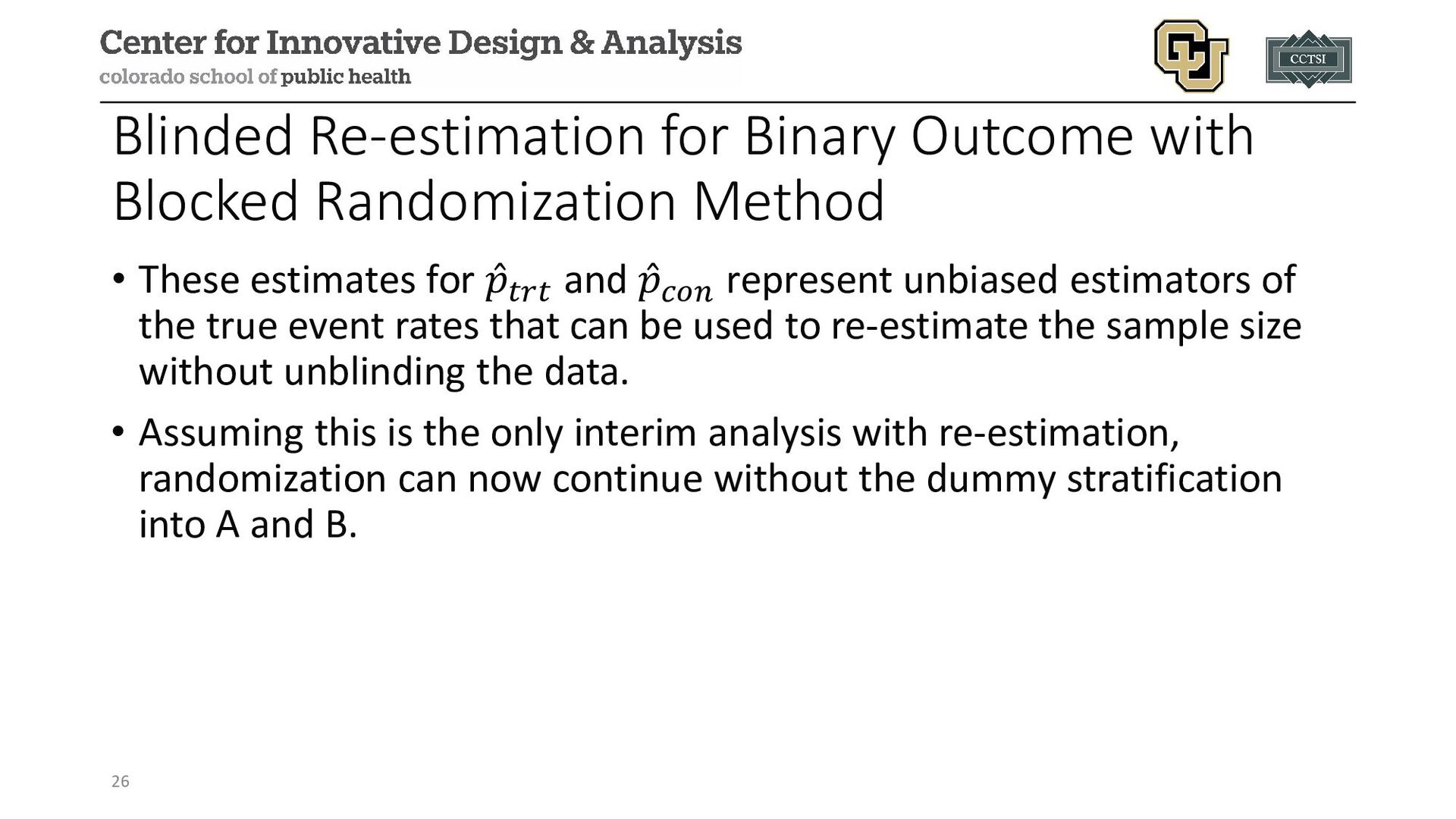
26. Blinded Re-estimation for Binary Outcome with Blocked Randomization Method • These estimates for ̂ 𝑝𝑝𝑡𝑡𝑡𝑡𝑡𝑡 and ̂ 𝑝𝑝𝑐𝑐𝑐𝑐𝑐𝑐 represent unbiased estimators of the true event rates that can be used to re-estimate the sample size without unblinding the data. • Assuming this is the only interim analysis with re-estimation, randomization can now continue without the dummy stratification into A and B. 26
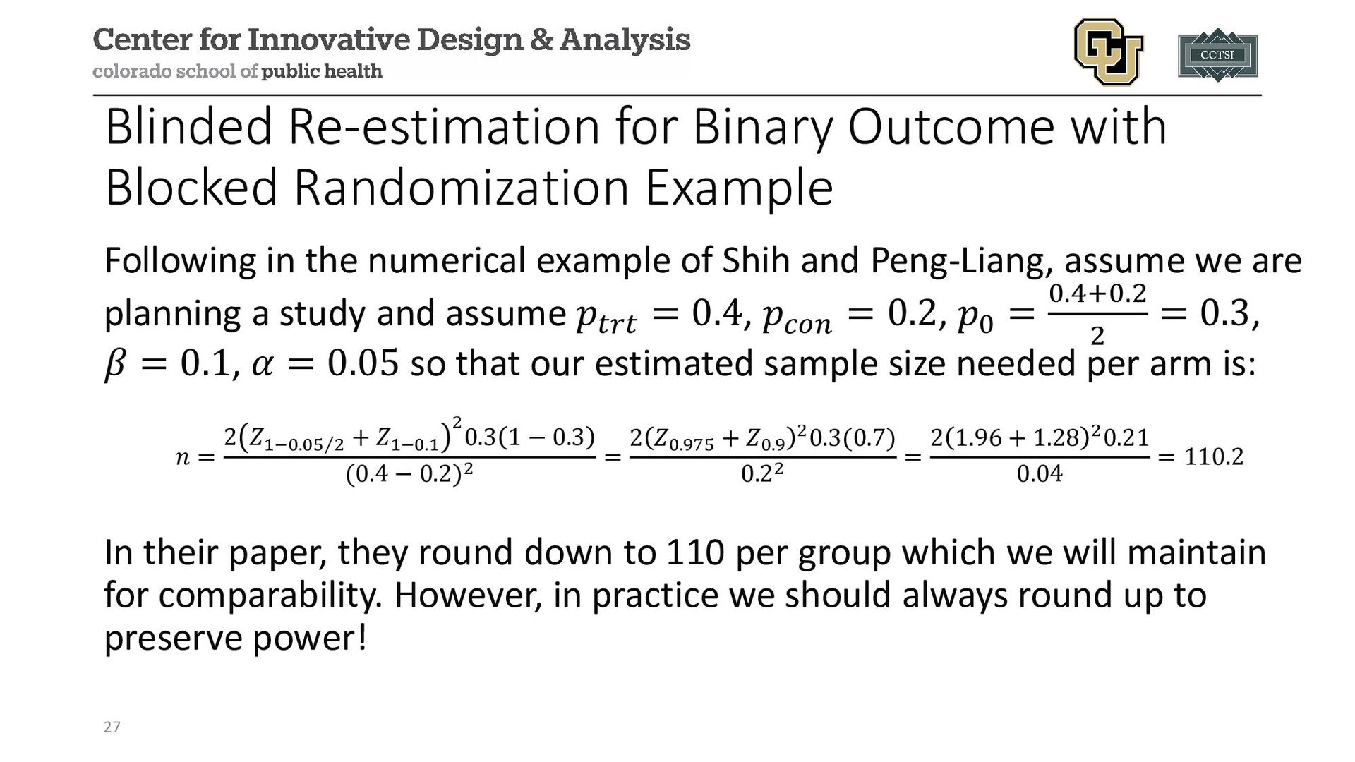
27. Blinded Re-estimation for Binary Outcome with Blocked Randomization Example Following in the numerical example of Shih and Peng-Liang, assume we are planning a study and assume 𝑝𝑝𝑡𝑡𝑡𝑡𝑡𝑡 = 0.4, 𝑝𝑝𝑐𝑐𝑐𝑐𝑐𝑐 = 0.2, 𝑝𝑝0 = 0.4+0.2 2 = 0.3, 𝛽𝛽 = 0.1, 𝛼𝛼 = 0.05 so that our estimated sample size needed per arm is: 𝑛𝑛 = 2 𝑍𝑍 ⁄ 1−0.05 2 + 𝑍𝑍1−0.1 2 0.3 1 − 0.3 (0.4 − 0.2)2 = 2 𝑍𝑍0.975 + 𝑍𝑍0.9 20.3(0.7) 0.22 = 2 1.96 + 1.28 20.21 0.04 = 110.2 In their paper, they round down to 110 per group which we will maintain for comparability. However, in practice we should always round up to preserve power! 27
28. Blinded Re-estimation for Binary Outcome with Blocked Randomization Example Let’s establish two dummy strata, A and B, with 𝜋𝜋 = 0.2. We know the strata allocation for each participant, but not their randomized treatment assignment. We have our interim analysis at 50% after 55 participants per strata and observe ̂ 𝜃𝜃1 = 0.28 and ̂ 𝜃𝜃2 = 0.37. We then plug into our equations: ̂ 𝑝𝑝𝑡𝑡𝑡𝑡𝑡𝑡 = 𝜋𝜋 � 𝜃𝜃1 − 1 − 𝜋𝜋 � 𝜃𝜃2 2𝜋𝜋 − 1 = 0.2 0.28 − 1 − 0.2 (0.37) 2 0.2 − 1 = 0.40 ̂ 𝑝𝑝𝑐𝑐𝑐𝑐𝑐𝑐 = 𝜋𝜋 � 𝜃𝜃2 − 1 − 𝜋𝜋 � 𝜃𝜃1 2𝜋𝜋 − 1 = 0.2 0.37 − 1 − 0.2 (0.28) 2 0.2 − 1 = 0.25 28
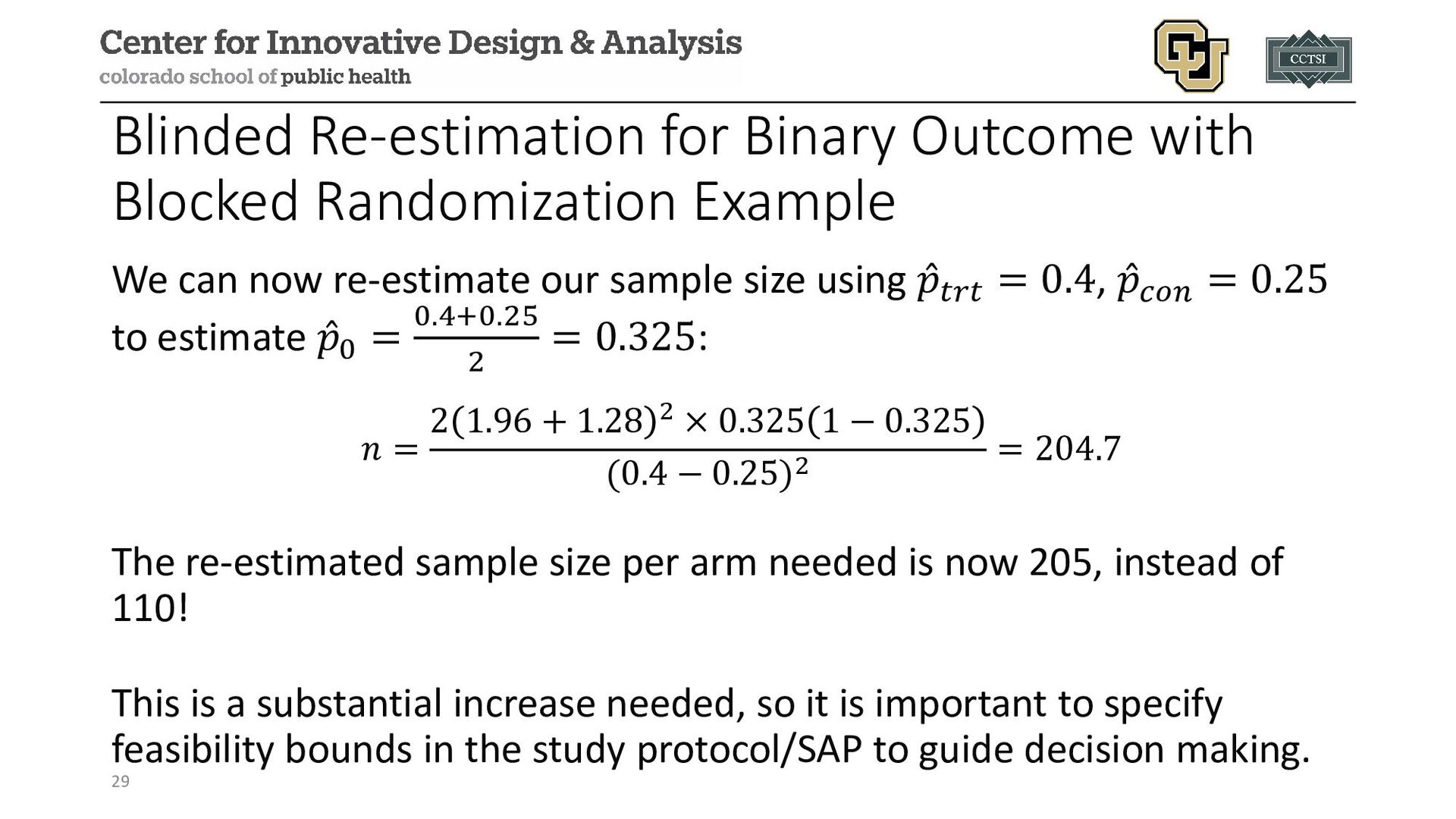
29. Blinded Re-estimation for Binary Outcome with Blocked Randomization Example We can now re-estimate our sample size using ̂ 𝑝𝑝𝑡𝑡𝑡𝑡𝑡𝑡 = 0.4, ̂ 𝑝𝑝𝑐𝑐𝑐𝑐𝑐𝑐 = 0.25 to estimate ̂ 𝑝𝑝0 = 0.4+0.25 2 = 0.325: 𝑛𝑛 = 2 1.96 + 1.28 2 × 0.325 1 − 0.325 (0.4 − 0.25)2 = 204.7 The re-estimated sample size per arm needed is now 205, instead of 110! This is a substantial increase needed, so it is important to specify feasibility bounds in the study protocol/SAP to guide decision making. 29
30. Unblinded Re-Estimation Methods Knowing the allocation, but inflating the risk of a type I error 30
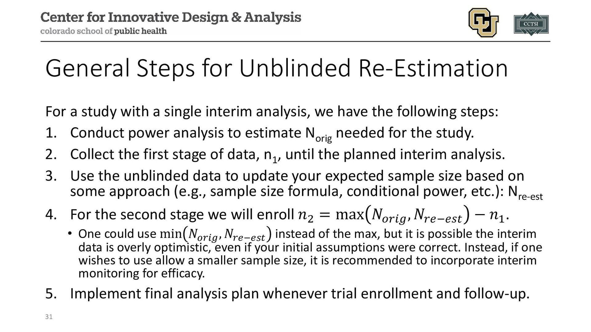
31. General Steps for Unblinded Re-Estimation For a study with a single interim analysis, we have the following steps: 1. Conduct power analysis to estimate Norig needed for the study. 2. Collect the first stage of data, n1 , until the planned interim analysis. 3. Use the unblinded data to update your expected sample size based on some approach (e.g., sample size formula, conditional power, etc.): Nre-est 4. For the second stage we will enroll 𝑛𝑛2 = max 𝑁𝑁𝑜𝑜𝑜𝑜𝑜𝑜𝑜𝑜 , 𝑁𝑁𝑟𝑟𝑟𝑟−𝑒𝑒𝑒𝑒𝑒𝑒 − 𝑛𝑛1. • One could use min 𝑁𝑁𝑜𝑜𝑜𝑜𝑜𝑜𝑜𝑜 , 𝑁𝑁𝑟𝑟𝑟𝑟−𝑒𝑒𝑒𝑒𝑒𝑒 instead of the max, but it is possible the interim data is overly optimistic, even if your initial assumptions were correct. Instead, if one wishes to use allow a smaller sample size, it is recommended to incorporate interim monitoring for efficacy. 5. Implement final analysis plan whenever trial enrollment and follow-up. 31
32. Type I Error Inflation • Unblinded re-estimation approaches may inflate the type I error rate because we observe the raw data and essentially are conducting a statistical test of significance via re-estimating the sample size • To maintain our trial operating characteristics, we need to consider statistical approaches that adjust for the unblinded re-estimation procedure in our final analysis plan. 32
33. Combination Tests • One strategy to control the type I error rate in an unblinded re- estimation procedure is to employ a combination test. • Many combination strategies have been proposed: • Inverse normal combination test (our focus on the next slides) • Inverse chi-squared test • Cauchy combination test • Fisher’s method 33
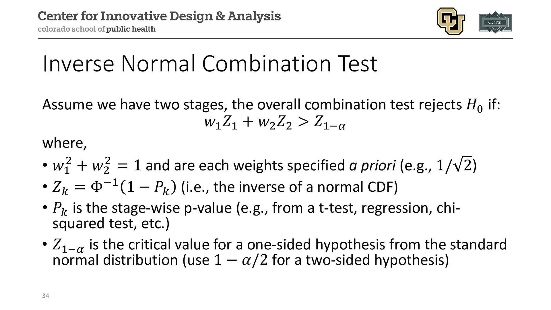
34. Inverse Normal Combination Test Assume we have two stages, the overall combination test rejects 𝐻𝐻0 if: 𝑤𝑤1 𝑍𝑍1 + 𝑤𝑤2 𝑍𝑍2 > 𝑍𝑍1−𝛼𝛼 where, • 𝑤𝑤1 2 + 𝑤𝑤2 2 = 1 and are each weights specified a priori (e.g., 1/ 2) • 𝑍𝑍𝑘𝑘 = Φ−1 1 − 𝑃𝑃𝑘𝑘 (i.e., the inverse of a normal CDF) • 𝑃𝑃𝑘𝑘 is the stage-wise p-value (e.g., from a t-test, regression, chi- squared test, etc.) • 𝑍𝑍1−𝛼𝛼 is the critical value for a one-sided hypothesis from the standard normal distribution (use 1 − 𝛼𝛼/2 for a two-sided hypothesis) 34
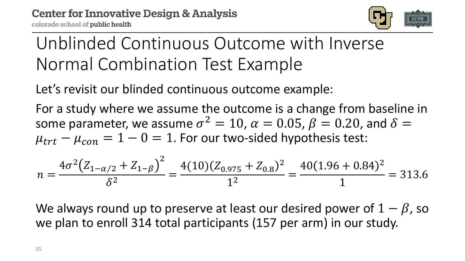
35. Unblinded Continuous Outcome with Inverse Normal Combination Test Example Let’s revisit our blinded continuous outcome example: For a study where we assume the outcome is a change from baseline in some parameter, we assume 𝜎𝜎2 = 10, 𝛼𝛼 = 0.05, 𝛽𝛽 = 0.20, and 𝛿𝛿 = 𝜇𝜇𝑡𝑡𝑡𝑡𝑡𝑡 − 𝜇𝜇𝑐𝑐𝑐𝑐𝑐𝑐 = 1 − 0 = 1. For our two-sided hypothesis test: 𝑛𝑛 = 4𝜎𝜎2 𝑍𝑍1− ⁄ 𝛼𝛼 2 + 𝑍𝑍1−𝛽𝛽 2 𝛿𝛿2 = 4(10) 𝑍𝑍0.975 + 𝑍𝑍0.8 2 12 = 40 1.96 + 0.84 2 1 = 313.6 We always round up to preserve at least our desired power of 1 − 𝛽𝛽, so we plan to enroll 314 total participants (157 per arm) in our study. 35
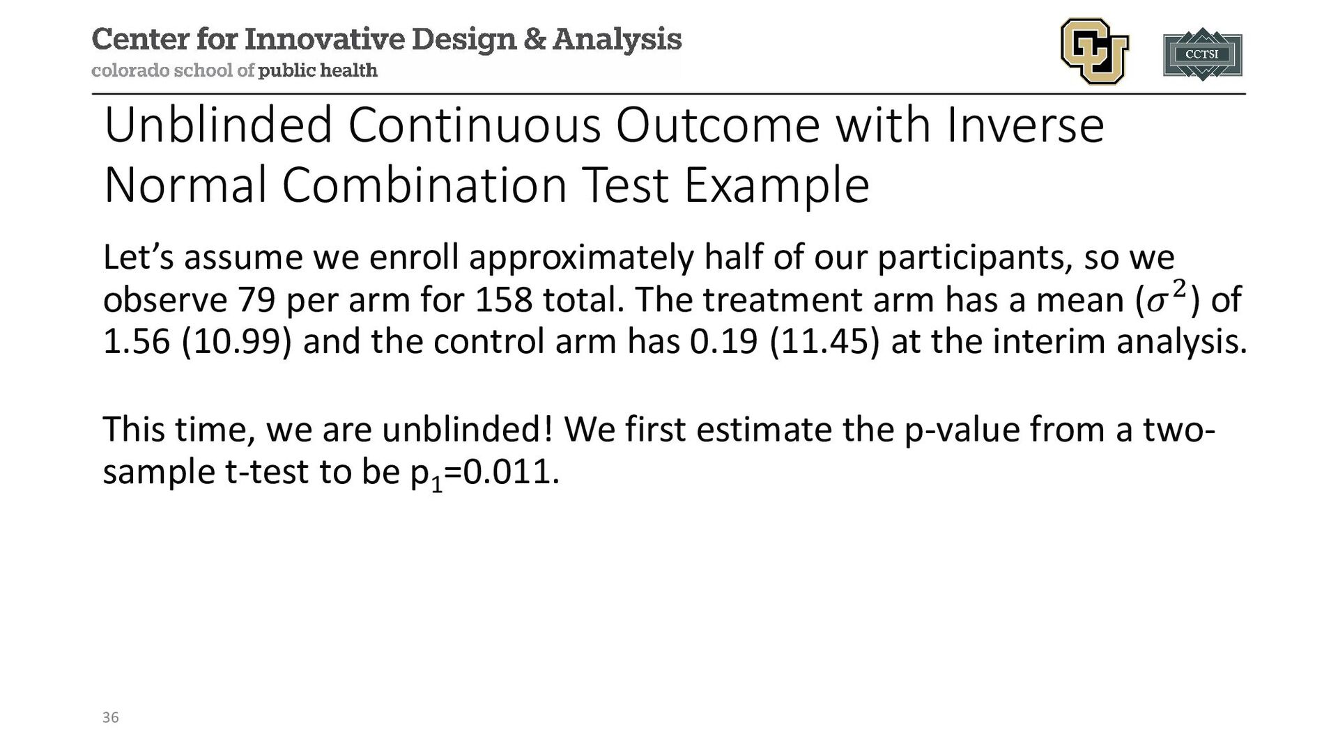
36. Unblinded Continuous Outcome with Inverse Normal Combination Test Example Let’s assume we enroll approximately half of our participants, so we observe 79 per arm for 158 total. The treatment arm has a mean (𝜎𝜎2) of 1.56 (10.99) and the control arm has 0.19 (11.45) at the interim analysis. This time, we are unblinded! We first estimate the p-value from a two- sample t-test to be p1 =0.011. 36
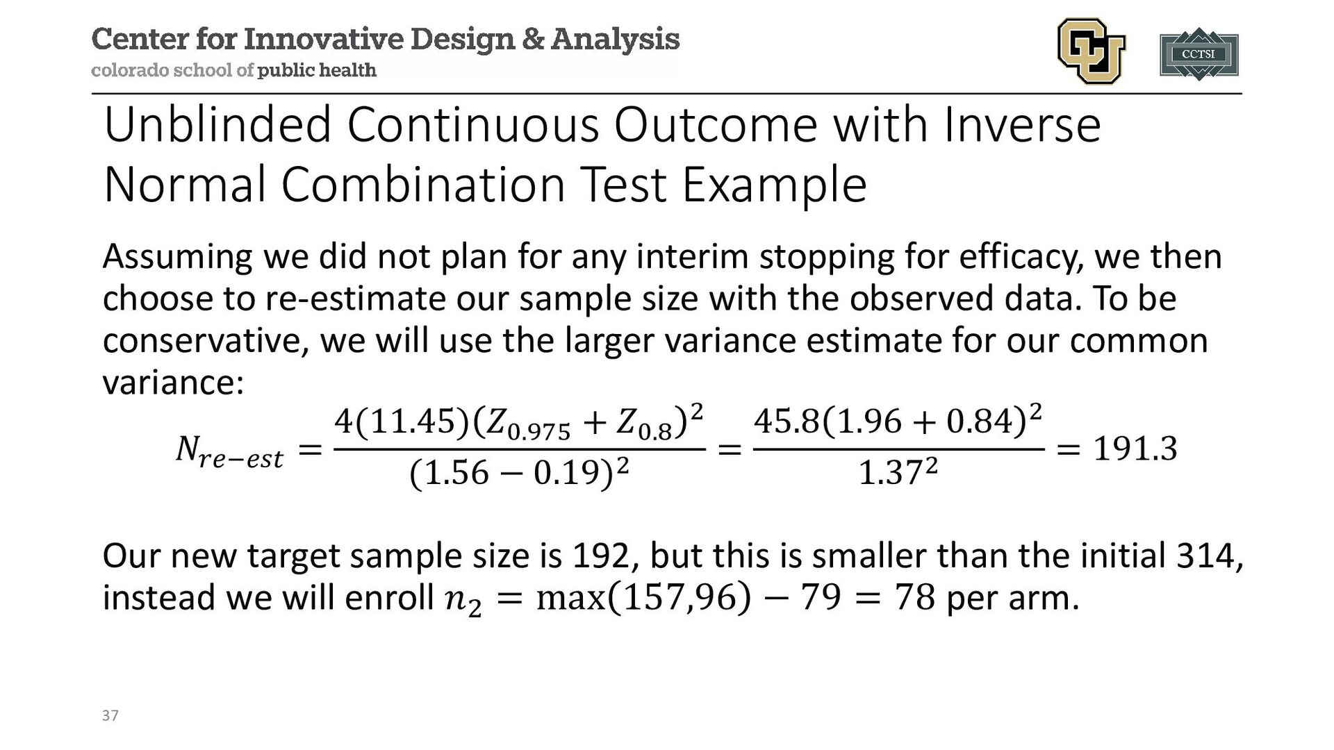
37. Unblinded Continuous Outcome with Inverse Normal Combination Test Example Assuming we did not plan for any interim stopping for efficacy, we then choose to re-estimate our sample size with the observed data. To be conservative, we will use the larger variance estimate for our common variance: 𝑁𝑁𝑟𝑟𝑟𝑟−𝑒𝑒𝑒𝑒𝑒𝑒 = 4(11.45) 𝑍𝑍0.975 + 𝑍𝑍0.8 2 (1.56 − 0.19)2 = 45.8 1.96 + 0.84 2 1.372 = 191.3 Our new target sample size is 192, but this is smaller than the initial 314, instead we will enroll 𝑛𝑛2 = max 157,96 − 79 = 78 per arm. 37
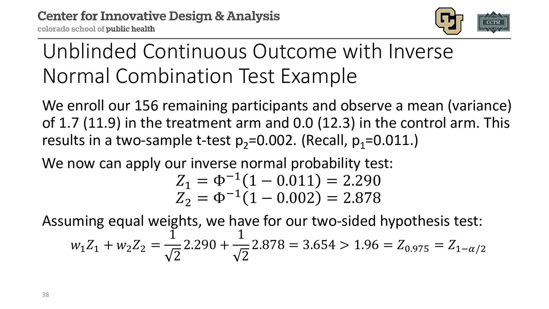
38. Unblinded Continuous Outcome with Inverse Normal Combination Test Example We enroll our 156 remaining participants and observe a mean (variance) of 1.7 (11.9) in the treatment arm and 0.0 (12.3) in the control arm. This results in a two-sample t-test p2 =0.002. (Recall, p1 =0.011.) We now can apply our inverse normal probability test: 𝑍𝑍1 = Φ−1 1 − 0.011 = 2.290 𝑍𝑍2 = Φ−1 1 − 0.002 = 2.878 Assuming equal weights, we have for our two-sided hypothesis test: 𝑤𝑤1 𝑍𝑍1 + 𝑤𝑤2 𝑍𝑍2 = 1 2 2.290 + 1 2 2.878 = 3.654 > 1.96 = 𝑍𝑍0.975 = 𝑍𝑍1−𝛼𝛼/2 38
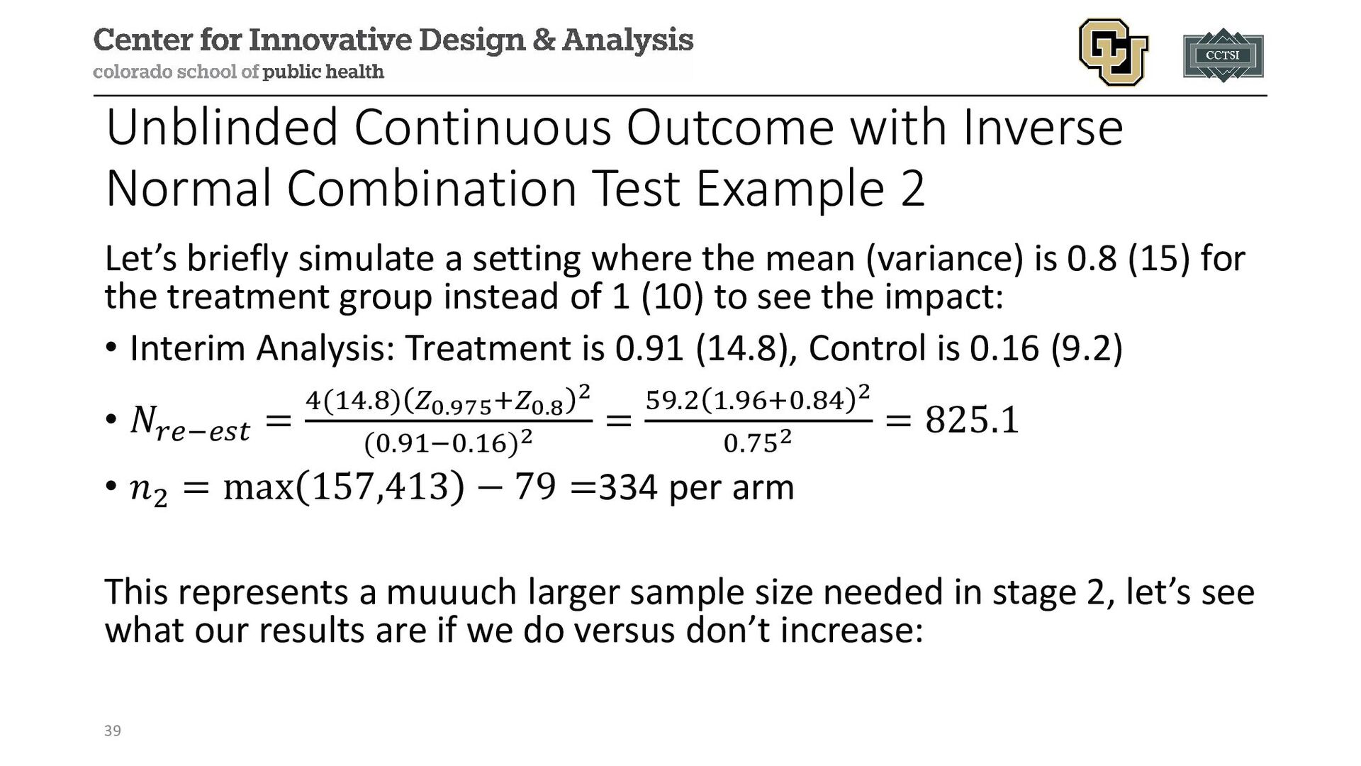
39. Unblinded Continuous Outcome with Inverse Normal Combination Test Example 2 Let’s briefly simulate a setting where the mean (variance) is 0.8 (15) for the treatment group instead of 1 (10) to see the impact: • Interim Analysis: Treatment is 0.91 (14.8), Control is 0.16 (9.2) • 𝑁𝑁𝑟𝑟𝑟𝑟−𝑒𝑒𝑒𝑒𝑒𝑒 = 4(14.8) 𝑍𝑍0.975+𝑍𝑍0.8 2 (0.91−0.16)2 = 59.2 1.96+0.84 2 0.752 = 825.1 • 𝑛𝑛2 = max 157,413 − 79 =334 per arm This represents a muuuch larger sample size needed in stage 2, let’s see what our results are if we do versus don’t increase: 39
40. Unblinded Continuous Outcome with Inverse Normal Combination Test Example 2 Original n2 =78 per arm: • Trt mean (var): 0.17 (13.4) • Con mean (var): -0.21 (8.8) • p1 =0.172, p2 =0.475 • 𝑍𝑍1 = Φ−1 1 − 0.172 = 0.946 • 𝑍𝑍2 = Φ−1 1 − 0.475 = 0.063 • 𝑍𝑍1+𝑍𝑍2 2 = 0.713 < 1.96 = Z0.975 • Fail to reject H0 Increased to n2 =334 per arm: • Trt mean (var): 0.93 (14.4) • Con mean (var): 0.24 (9.2) • p1 =0.172, p2 =0.0099 • 𝑍𝑍1 = Φ−1 1 − 0.172 = 0.946 • 𝑍𝑍2 = Φ−1 1 − 0.0099 = 2.33 • 𝑍𝑍1+𝑍𝑍2 2 = 2.316 > 1.96 = Z0.975 • Reject H0 , difference in arms 40
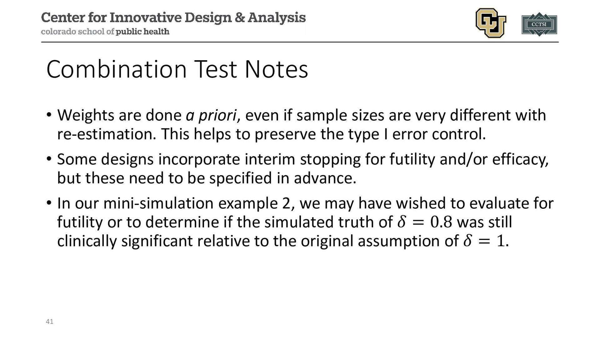
41. Combination Test Notes • Weights are done a priori, even if sample sizes are very different with re-estimation. This helps to preserve the type I error control. • Some designs incorporate interim stopping for futility and/or efficacy, but these need to be specified in advance. • In our mini-simulation example 2, we may have wished to evaluate for futility or to determine if the simulated truth of 𝛿𝛿 = 0.8 was still clinically significant relative to the original assumption of 𝛿𝛿 = 1. 41
42. Conditional Power/Predictive Power for Re- Estimation • It is also possible to use the frequentist conditional power or Bayesian predictive power (also called the predictive posterior probability of success or the probability of success (PPoS)) for re-estimation • At the interim analysis, the sample size needed to achieve a targeted conditional power is detected (e.g., via a grid search or other software) • These methods still require some form of correction for multiple testing (e.g., combination test for final inference) • As with any study design, operating characteristics can be evaluated via simulation studies 42
43. Case Studies 43
44. Clinical Trial: Sample Size Re-Estimation Example I Name: Tenecteplase versus Alteplase before Endovascular Therapy for Ischemic Stroke (EXTEND-IA TNK) (NCT02388061) Design: multi-center, randomized, open-label, non-inferiority, blinded- outcome Population: ischemic stroke within 4.5 hours after onset and eligible to undergo intravenous thrombolysis and endovascular thrombectomy Purpose: compare intravenous tenecteplase with alteplase to evaluate non-inferiority, then potentially superiority, of tenecteplase 44
45. Clinical Trial: Sample Size Re-Estimation Example I N: 120 based on initial power calculation for 80% power, but substantial uncertainty over participant disposition and prevalence of outcome Randomization Ratio: 1:1 Primary Outcome: proportion of participants with restoration of blood flow to >50% of the affected arterial territory or absence of retrievable thrombus at initial angiogram Re-Estimation Approach: blinded re-estimation 45
46. Clinical Trial: SSR Example I Conclusion • Blinded re-estimation approach implemented after enrollment of 100 participants • Re-estimated sample size was 202 participants to establish non- inferiority, a 68% increase from initial estimate of 120 • Trial continued to enroll a total of 202 participants, 101 in each arm • Ultimately determined that tenecteplase (22% event rate) was non- inferior to alteplase (10% event rate) 46
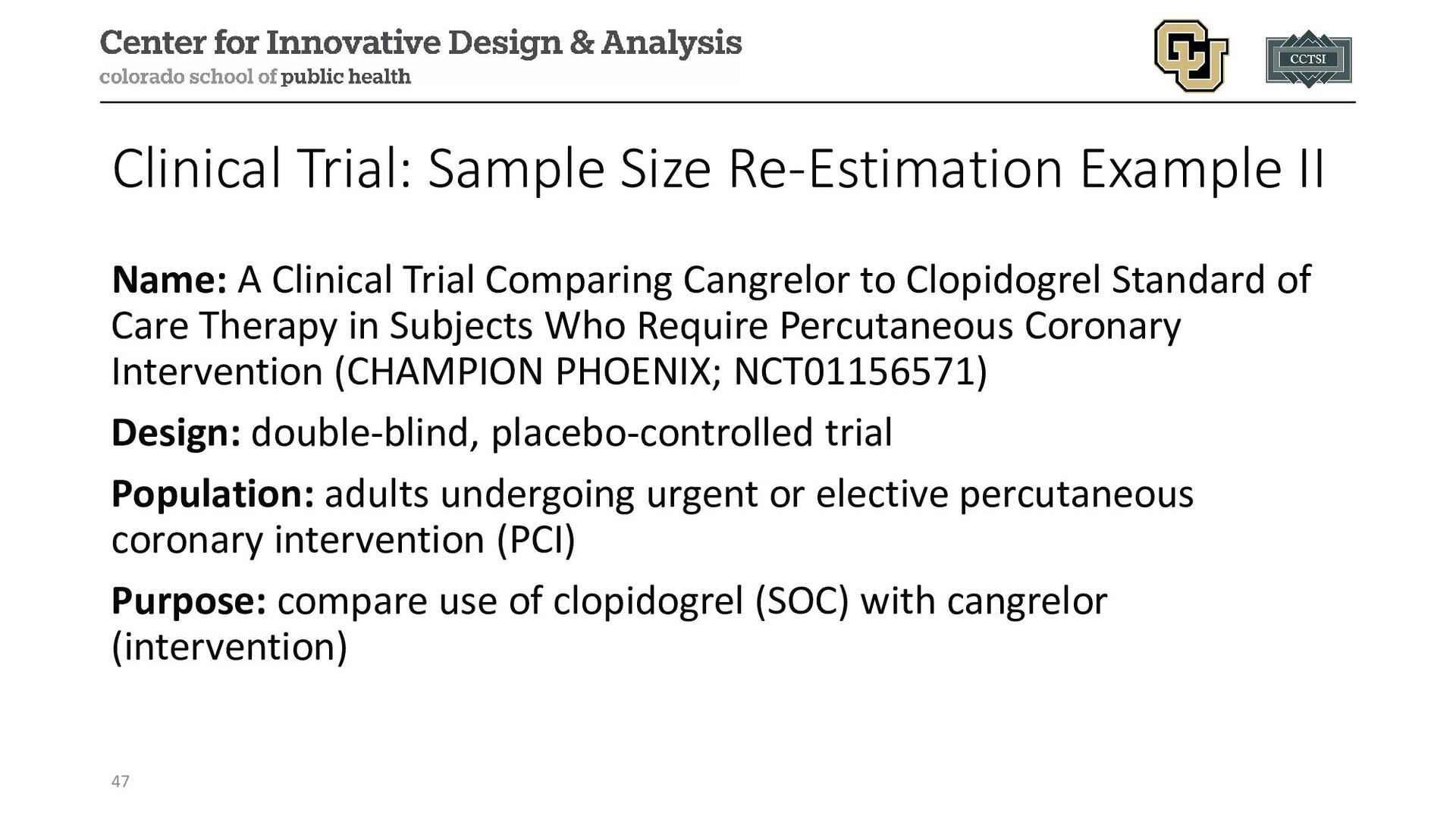
47. Clinical Trial: Sample Size Re-Estimation Example II Name: A Clinical Trial Comparing Cangrelor to Clopidogrel Standard of Care Therapy in Subjects Who Require Percutaneous Coronary Intervention (CHAMPION PHOENIX; NCT01156571) Design: double-blind, placebo-controlled trial Population: adults undergoing urgent or elective percutaneous coronary intervention (PCI) Purpose: compare use of clopidogrel (SOC) with cangrelor (intervention) 47
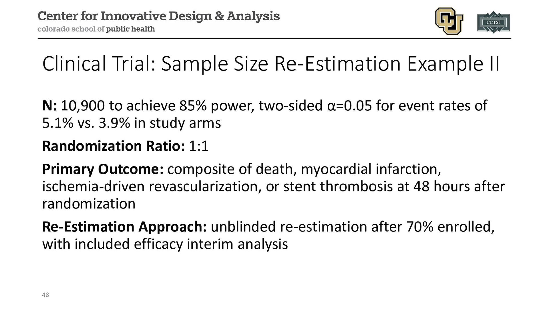
48. Clinical Trial: Sample Size Re-Estimation Example II N: 10,900 to achieve 85% power, two-sided α=0.05 for event rates of 5.1% vs. 3.9% in study arms Randomization Ratio: 1:1 Primary Outcome: composite of death, myocardial infarction, ischemia-driven revascularization, or stent thrombosis at 48 hours after randomization Re-Estimation Approach: unblinded re-estimation after 70% enrolled, with included efficacy interim analysis 48
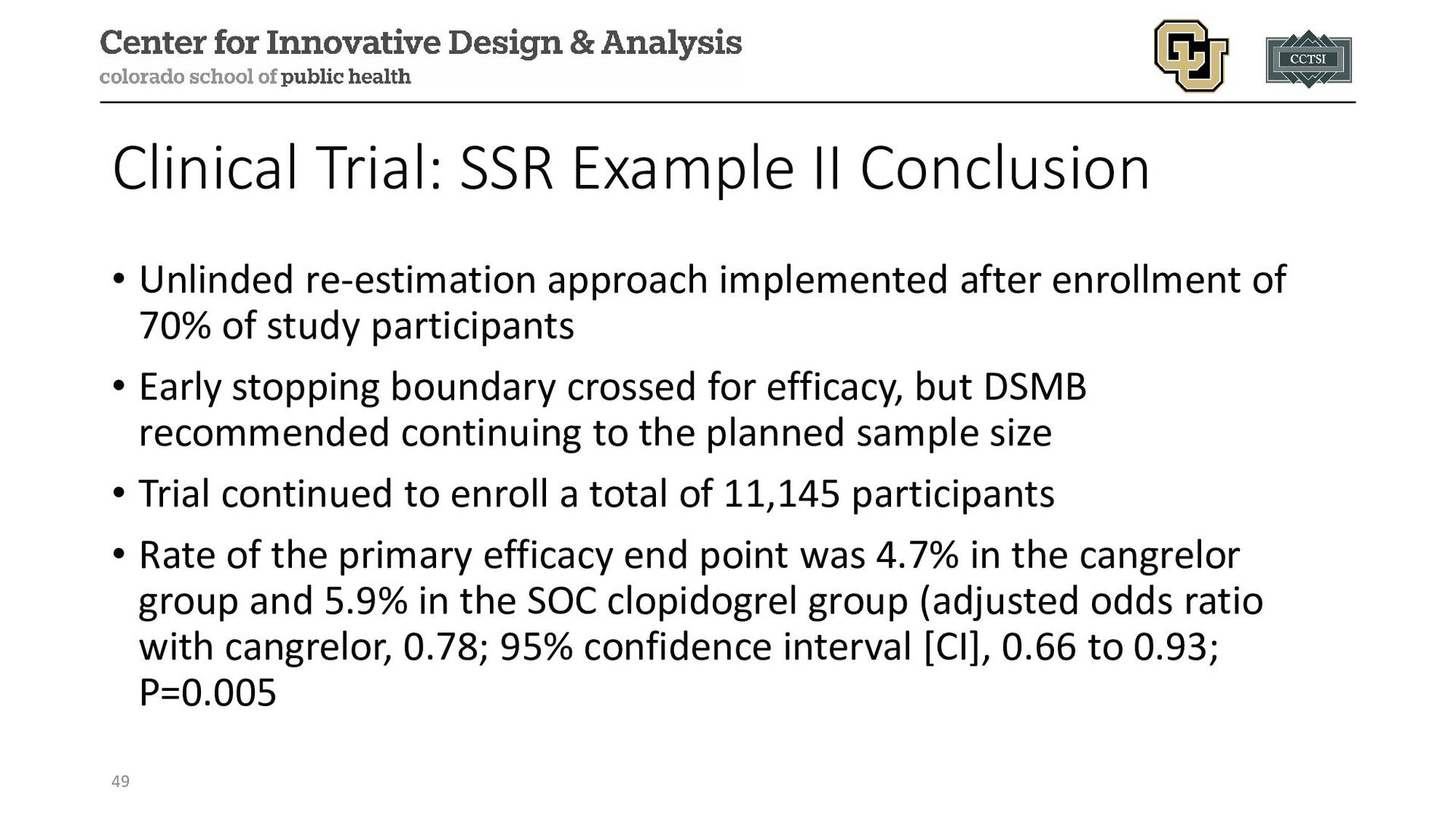
49. Clinical Trial: SSR Example II Conclusion • Unlinded re-estimation approach implemented after enrollment of 70% of study participants • Early stopping boundary crossed for efficacy, but DSMB recommended continuing to the planned sample size • Trial continued to enroll a total of 11,145 participants • Rate of the primary efficacy end point was 4.7% in the cangrelor group and 5.9% in the SOC clopidogrel group (adjusted odds ratio with cangrelor, 0.78; 95% confidence interval [CI], 0.66 to 0.93; P=0.005 49
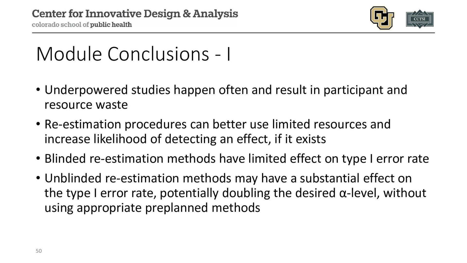
50. Module Conclusions - I • Underpowered studies happen often and result in participant and resource waste • Re-estimation procedures can better use limited resources and increase likelihood of detecting an effect, if it exists • Blinded re-estimation methods have limited effect on type I error rate • Unblinded re-estimation methods may have a substantial effect on the type I error rate, potentially doubling the desired α-level, without using appropriate preplanned methods 50
51. Module Conclusions - II • Practical considerations should be considered and included in the protocol for how much of a sample size change would be feasible or possible (e.g., budget, timeframe, patient population, minimal effect size of interest, etc.) • Care should be taken in reporting interim results, since it may be possible to back-calculate the effect size if one knows general assumptions (resulting in an accidental unblinding) • Possible to combine re-estimation with stopping for futility, efficacy, or safety, as well as other adaptive methods • We only consider a small subset of methods, and more exist to explore and consider 51
52. References • Ciolino, Jody D., Alexander M. Kaizer, and Lauren Balmert Bonner. "Guidance on interim analysis methods in clinical trials." Journal of Clinical and Translational Science 7.1 (2023): e124. • Kaizer, Alexander M., et al. "Recent innovations in adaptive trial designs: a review of design opportunities in translational research." Journal of Clinical and Translational Science (2023): 1-35. • Proschan, Michael A. "Sample size re‐estimation in clinical trials." Biometrical Journal: Journal of Mathematical Methods in Biosciences 51.2 (2009): 348-357. • Baumann, Lukas, Maximilian Pilz, and Meinhard Kieser. "blindrecalc-An R Package for Blinded Sample Size Recalculation." R Journal 14.1 (2022). • Fleiss, Joseph L., Bruce Levin, and Myunghee Cho Paik. Statistical methods for rates and proportions. John Wiley & Sons, 2013. • Shih, Weichung Joseph, and Peng‐Liang Zhao. "Design for sample size re‐estimation with interim data for double‐blind clinical trials with binary outcomes." Statistics in Medicine 16.17 (1997): 1913-1923. • Campbell, Bruce CV, et al. "Tenecteplase versus alteplase before thrombectomy for ischemic stroke." New England Journal of Medicine 378.17 (2018): 1573-1582. • Bhatt, Deepak L., et al. "Effect of platelet inhibition with cangrelor during PCI on ischemic events." New England Journal of Medicine 368.14 (2013): 1303-1313. • Leonardi, Sergio, et al. "Rationale and design of the Cangrelor versus standard therapy to acHieve optimal Management of Platelet InhibitiON PHOENIX trial." American heart journal 163.5 (2012): 768-776. • US Food and Drug Administration. Adaptive designs for clinical trials of drugs and biologics guidance for industry. https://www.fda.gov/regulatory-information/search-fda-guidance-documents/adaptive-design-clinical-trials-drugs-and-biologics-guidance- industry
53. Contact Info: • Email: • alex.kaizer@cuanschutz.edu • Website: www.alexkaizer.com • GitHub: alexbiostats